Background
Need for Advanced Detection Systems
In recent years, the rise of internet and cloud technologies has significantly increased the volume of online purchases and transactions. This expansion has led to unauthorized access to sensitive user information and compromised enterprise resources. Phishing, a common type of attack, deceives users into accessing malicious content to steal their information (Dutta, 2021).
Often, phishing websites mimic legitimate ones in terms of their interface and URL (Levy, 2004).
Various methods, including blacklists and heuristic approaches, have been proposed to detect these phishing sites. However, heuristics are more effective in detecting phishing sites than blacklists due to their short lifetime and ability to distinguish legitimate from phishing sites (Gastellier-Prevost, 2011).
Current research indicates that the effectiveness of phishing detection systems is limited, highlighting the need for more advanced, intelligent techniques to safeguard users against these cyber threats (Dutta, 2021).
A Machine Learning Approach: Idea Formulation
ML models can learn from large amounts of data to recognize patterns that are typical of phishing sites.
Consider two URLs:
https://upenn-payments.xyz/payment.phpandhttps://srfs.upenn.edu/billing-payment/pennpay.
At first glance to an unsuspecting user, both might appear legitimate, but a ML model can be trained to detect phishing to evaluate their features. For instance, the domain name penn-payments.xyz might raise red flags as it uses a less common and perhaps sketchy top-level domain (.xyz) compared to the more trusted .edu TLD in srfs.upenn.edu.
)](https://raw.githubusercontent.com/jimyy23/pennfish-hugo/refs/heads/master/content/post/report/Untitled.png)
Source: MDN (https://developer.mozilla.org/en-US/docs/Learn/Common_questions/Web_mechanics/What_is_a_URL)
Moreover, the first URL is shorter and lacks a path structure that implies a deeper, more organized content hierarchy as seen in the second URL with /billing-payment/pennpay.
Our assumption is that by extracting and analyzing these URL features, a machine learning model can learn to predict potential phishing threats with greater accuracy, providing a feasible and powerful tool in cybersecurity efforts.
We plan to use ML models to leverage these features to scrutinize URLs and identify potential phishing threats.
Project Overview
In our project, we've used a number of machine learning approaches.
Here’s a brief overview:
- Data Pre-processing - we started the project with cleaning the data and exploring additional sources of data that we can integrate into the original dataset.
- Exploratory Data Analysis (EDA) - we explored the data to understand the characteristics and patterns that might be present.
- Feature Engineering - We modify features from the existing data to better extract patterns that can be important for phishing detection.
- Linear Regression (Unregularized) - This is a basic approach where we try to fit a straight line that predicts phishing likelihood based on input features.
- Ridge Regression - To analyze data that suffers from multicollinearity (when independent variables are highly correlated).
- Logistic Regression - A step up from linear regression, this method is specifically used for binary classification tasks like ours (phishing or not).
- PCA to Reduce Dimensionality, Logistic Regression with PCA - This approach first reduces the complexity of the data using Principal Component Analysis (PCA) and then applies logistic regression to the simplified data.
- Decision Tree Classifier - We used it to makes decisions based on asking a series of specific questions about the features of the URL.
- Random Forest Classifier - An ensemble method that uses multiple decision trees to improve the classification accuracy.
- SVM (Support Vector Machine) - A more sophisticated classification technique that finds the best boundary to differentiate between phishing and non-phishing URLs.
- Artificial Neural Network Model - We ended the project by leveraging ANN to model and predict phishing URLs, capable of capturing intricate patterns in the data.
Dive into the Datasets
UCI Machine Learning Repository
Dataset Selection
For our project on detecting phishing URLs, we chose a dataset crafted by Arvind Prasad and Shalini Chandra, as detailed in their paper titled "PhiUSIIL: A diverse security profile empowered phishing URL detection framework based on similarity index and incremental learning."
This data set was released in March 2024.
This dataset is specifically created for the task of phishing URL detection and includes a robust framework that leverages a similarity index. This index is quite effective in identifying visual similarity-based attacks, such as those involving zero-width characters, homographs, punycode, homophones, bit squatting, and combosquatting.
We selected this dataset because of its richness and the extensive range of features it offers, which are not typically available in more generic datasets such as similar ones from Kaggle.
Features of the Original Dataset
Let's check the first few rows of the dataset.
df_features.head(2)
The author of this dataset has described the features in the dataset as follows:
TLD: TLD (Top Level Domain) is the last part of the domain name, such as .com or .edu. Phishing URLs often use TLDs that are not commonly associated with the legitimate domain, such as .link or .inf.URLLength: Phishing URLs are often longer than legitimate URLs as they contain additional digits, symbols, subdirectories, and parameters.IsDomainIP: a URL using an IP address instead of a domain name can be a red flag for users.NoOfSubDomain: Subdomain is part of URL that appears before domain name. Cybercriminals often use visual similarity techniques to trick users. They create subdomains that look like subdomain of legitimate websites.NoOfObfuscatedChar: Shows a count of obfuscated characters in URL.IsHTTPS: Indicates if the webpage is running on unsecured HTTP (hypertext transfer protocol) or secured HTTPS. A URL using the http protocol is highly likely to be a phishing URL. Most legitimate websites, especially those that require users to input sensitive information like passwords or credit card numbers, use HTTPS to protect their users’ data. If a webpage asks for sensitive information but doesn’t use HTTPS, it could be a sign that the webpage is a phishing scam.- No. of digits, equal, qmark, amp: A large number of digits or symbols such as ‘=’, ‘?’, or ‘%’ in a URL increases the possibility of being a phishing URL.
HasFavicon: Most legitimate websites have their website logo included in the favicon tag. Missing a favicon tag may indicate a phishing scam.IsResponsive: Most legitimate websites are responsive, which helps web content to be appropriately adapted across devices to give better readability and view. Fortunately, many phishing websites are not responsive, as threat actors find it challenging to ensure the responsiveness of their quickly designed websites on all major devices.NoOfURLRedirect: Phishing sites may use redirects to direct users to a different page than they were expecting. For example, the HTML code may contain JavaScript or meta tags that redirect users to a different URL. The HTML tags such as ‘http-equiv’, ‘refresh’, ‘window.location’, ‘window.location.replace’, ‘window.location-.href’, ‘http.open’ can help identify URL redirection.HasDescription: Legitimate websites provide page descriptions for each page using the ‘description’ meta name. Missing page descriptions may raise a red flag for a webpage.NoOfPopup,NoOfiFrame: Phishing websites may use pop-ups or iframe to distract users and capture sensitive information. These pop-ups and iframe can be detected by looking for tags ‘window.open’ and ‘iframe’ in the HTML code.HasExternalFormSubmit: Phishing sites often use HTML forms to collect user information. Form submitting to an external URL can be a red flag for users.HasCopyrightInfo, HasSocialNet: Most legitimate websites have copyright and their social networking information. Missing such information may indicate a phishing scam.HasPasswordField, HasSubmitButton: HTML provides a variety of form elements that allow users to input data and submit it to other URLs. For example, HTML tags such as ‘passwordfield’ or ‘submitbutton’ can be extracted to examine the HTML code of the webpage.HasHiddenFields: Phishing websites may use hidden fields to capture sensitive information without the user’s knowledge. These fields can be detected by examining the HTML code of the webpage.Bank,Pay,Crypto: Elements such as bank, pay, or crypto may indicate that the webpage is asking for sensitive financial information from the user, which may be used to siphon money. Therefore, such websites need to be analyzed for suspicious activities.NoOfImage: Threat actors can use screenshots of legitimate websites and design phishing websites to make them appear more legitimate. More images used in respectively small websites may indicate phishing websites.NoOfJS: JavaScript is a programming language that can be embedded in HTML to create interactive webpages. Phishing websites may use JavaScript to create pop-up windows or other misleading elements that trick users into revealing sensitive information. A large number of JavaScript included in a webpage can make it suspicious.NoOfSelfRef,NoOfEmptyRef,NoOfExternalRef: Hyperlinks (href) are clickable links that allow users to navigate between webpages or navigate to external webpages. Phishing websites may use hyperlinks that appear to direct to a legitimate webpage, but instead, they redirect the user to a phishing page. A large number of hyperlinks navigating to itself, navigating to empty links, or navigating to external links can be suspicious.URLTitleMatchScore: Cybercriminals often use social engineering tactics to trick users into believing a website is legitimate. They may use a URL that looks similar to a legitimate website and create a convincing webpage title reflecting the website’s content. We introduced URLTitleMatchScore to identify the discrepancy between the URL and the webpage title. A lower score can be a sign that the website is a phishing attempt because the webpage title does not match the content that is expected to be found on the website. A higher score 100 or close to 100 indicates that the website is what it claims to be. The code to calculate URLTitleMatchScore is given in Algorithm 1.URLCharProb: While most legitimate URLs look meaningful, many phishing URLs contain random alphabet, digits, and misspelled words that do not look meaningful. Often, an attacker uses the typosquatting technique to create a URL similar to a legitimate URL but with small typographical errors. To understand the pattern of each alphabet and digit in a URL, we count the occurrence of each alphabet and digit in the 10 million legitimate URLs and divide them by the total count of all alphabets and digits of 10 million legitimate URLs. Further, to compare it with the pattern of phishing URLs, we collected 7 million phishing URLs and calculated the probability of each alphabet and digit using the same method. The probability of each alphabet and digit calculated from the 10 million legitimate URLs is used to calculate the URLCharProb of a URL by combining the probability of each alphabet and digit and dividing it by the URL length. The formula to calculate the URLCharProb of each URL is given below.
$$ URLCharProb = \sum_{i=0}^{n} \frac{\text{prob}(URLChar_i)}{n} $$
TLDLegitimateProb: The top-level domain (TLD) is the last part of a domain name that indicates the purpose or origin of a URL. Phishing attackers often use TLDs that are uncommon or unrelated to the purpose of the website they are trying to spoof. Legitimate websites often use specific TLDs associated with their industry or location. We extracted all the TLDs from the top 10 million websites and counted the occurrence of each TLD. Further, we calculated the ratio of each TLD by dividing the total occurrence of that TLD by the total occurrence of all the TLDs. A higher TLDLegitimateProb of a URL may indicate a legitimate URL, and a lower TLDLegitimateProb value may help identify phishing URLs. In summary, the phishing URL dataset construction technique involves extracting and analyzing the URL, HTML, and derived features to create a comprehensive dataset for detecting phishing attacks. These features provide valuable information about the potential malicious intent of the URL.
Data Cleaning
Some TLDs have port numbers such as com:4000 which is not appropriate for the TLD fields. We removed the port numbers from the TLDs.
## Remove any port number
df_features['TLD'] = df_features['TLD'].str.split(':').str[0]
The TLD field appears to be extracting everything after the last dot. However, this resulted in invalid TLDs such as '45' because an URL could be just an IP address.
We fixed this by replacing any numeric TLDs with 'ip' for the sake of our analysis. 'ip' is not a valid TLD, but it will help us identify IP addresses.
## Replace numeric TLDs with 'ip'
df_features['TLD'] = df_features['TLD'].apply(lambda x: 'ip' if x.isnumeric() else x)
Finally, let’s check the nulls and duplicates:
num_nulls = df_urls_data.isnull().sum().sum()
print(f"Number of null values: {num_nulls}")

num_dups = df_urls_data.duplicated().sum()
print(f"Number of duplicated values: {num_dups}")
Upon examining the dataset, we found no null values and duplicates. Deduplication is not needed.
We can proceed to the next steps!
Integrating the Public Suffix List Data
The TLD field currently in the dataset only contains the top-level-domains. However, we need to extract the public suffixes from the URLs. We will use the publicsuffix2 package to extract the public suffixes from the URLs.
## Install the publicsuffix2 package
## Usage: https://pypi.org/project/publicsuffix2/
!pip install publicsuffix2
What is the PSL?
A "public suffix" is one under which Internet users can (or historically could) directly register names. Some examples of public suffixes are .com, .co.uk and pvt.k12.ma.us. The Public Suffix List is a list of all known public suffixes.
It allows browsers to, for example:
- Avoid privacy-damaging "supercookies" being set for high-level domain name suffixes
- Highlight the most important part of a domain name in the user interface
- Accurately sort history entries by site
The Public Suffix List is an initiative of Mozilla, but is maintained as a community resource. It is available for use in any software, but was originally created to meet the needs of browser manufacturers.
- The PSL project website: https://publicsuffix.org
The Public Suffix List is playing a crucial role in the operation of the Internet, yet it's maintained by a small team toiling in obscurity.
- Interesting to read: The Present and Future of the Public Suffix List
What is eTLD?
The PSL is a list of domain names that are controlled by a single organization.
For example, co.uk is a PSL domain, but uk is a TLD.
In Japan, while jp is a TLD, co.jp and ne.jp is an effective TLD. Japan even has city-level eTLDs like tokyo.jp.
The PSL is useful for extracting the root domain from a URL.
Here is a visualization of the hierarchy of some more examples:
)](https://raw.githubusercontent.com/jimyy23/pennfish-hugo/refs/heads/master/content/post/report/Untitled_3.png)
Source: Steve Jones (https://www.linkedin.com/pulse/public-suffix-list-needs-support-we-also-need-something-steve-jones)
EDA implications
In the EDA section, we are also going to explore the pricing of domain names. The PSL is useful for this analysis because the prices are different for second-level domains (SLDs) and top-level domains (TLDs) in some cases. For example, the price of .co.uk may be different from .uk.
Integrating the PSL Data
psl = PublicSuffixList()
## Extract the domain and second level domain (SLD)
def extract_domain_and_sld(url):
parsed_url = urlparse(url)
domain = parsed_url.netloc
if not domain:
domain = url.split('/')[0] #passed directly as domain names
# Strip away port numbers and username/password in URL
domain = domain.split('@')[-1].split(':')[0]
# Replace any backslashes
domain = domain.replace('\\', '/').split('/')[0]
# Use publicsuffix2 to extract the second level domain (SLD)
tld = get_tld(domain)
return {'domain': domain, 'tld': tld}
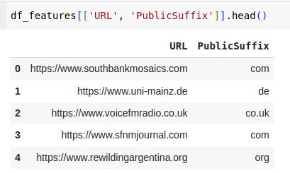
## Extract the eTLD
df_features['PublicSuffix'] = df_features['URL'].apply(lambda x: extract_domain_and_sld(x)['tld'])Make sure the public suffixes have been extracted properly:
## List the unique values of PublicSuffix
unique_ps = df_features['PublicSuffix'].unique()
print(f"Unique PublicSuffix: {unique_ps}")

## Check for null values
num_nulls_ps = df_features['PublicSuffix'].isnull().sum()
print(f"Number of null in PublicSuffix: {num_nulls_ps}")

## Output: Number of null in PublicSuffix: 0
Integrating the Domain Pricing Data
Background on Pricing of Domain Names
How domains are acquired?
The domains are acquired through domain registrars. The domain registrars are mostly accredited by the registries. The domain registrars are responsible for selling domain names to the public.
Note - difference between registrar and registry: The registry is responsible for managing the top-level domain (TLD) and the registrar is responsible for selling the domain names to the public.
)](https://raw.githubusercontent.com/jimyy23/pennfish-hugo/refs/heads/master/content/post/report/Untitled_5.png)
Source: Cloudflare (https://www.cloudflare.com/learning/dns/glossary/what-is-a-domain-name-registrar/)
So, at what price are domains sold?
The domain prices are set by the domain registrars. The prices vary depending on the domain extension. For example, '.com' domains are generally more expensive than '.xyz' domains. So, that makes '.xyz' more likely to be used by phishers.
Acquire Pricing Data of Domain Names
Since different domain registrar charges prices differently even for the same domain suffix. For example, GoDaddy sells .com more expensive than Namecheap.
We assume that the phisers want to save money and they will choose the cheapest domain registrar to buy the domain. So, we will use the cheapest price of the domain suffix as the price of the domain suffix available in the market.
Acquiring the Domain Market Data
One of the best sources for domain pricing data is the domain registrars themselves. We will use the tld-list.com platform, which provides domain pricing data for various domain registrars.
)](https://raw.githubusercontent.com/jimyy23/pennfish-hugo/refs/heads/master/content/post/report/Untitled_6.png)
Source: TLD-list (https://tld-list.com)
The data has been dumped from the tld-list.com platform and stored in a Cloudflare R2 storage bucket. We will download the data and load it into a dataframe.
## Load the TLD pricing data
df_tld_pricing = pd.read_csv('tld-pricing.csv')
df_tld_pricing.head()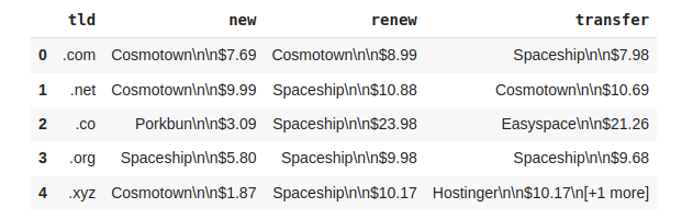
Obviously, we need to perform some data cleaning work.
## remove anything before '$' for all cols and all rows
df_tld_pricing['new'] = df_tld_pricing['new'].str.extract(r'(\d+\.\d+)').astype(float)
df_tld_pricing = df_tld_pricing.drop(columns=['renew', 'transfer'])
df_tld_pricing = df_tld_pricing.reset_index(drop=True)

## get rid of the first dot in tld, if exists
df_tld_pricing['tld'] = df_tld_pricing['tld'].str.replace('.', '', 1)

## df_tld_pricing.head()

## rename columns 'new': 'DomainPrice', 'tld': 'PublicSuffix'
df_tld_pricing.columns = ['PublicSuffix', 'DomainPrice']

## drop any rows missing 'new' price
df_tld_pricing = df_tld_pricing.dropna(subset=['DomainPrice'])
df_tld_pricing = df_tld_pricing[df_tld_pricing['DomainPrice'] > 0] # keep only > 0 prices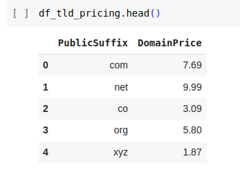
There are certain suffixes of which a domain price is not available due to many reasons. We impute these values with the median domain price, which is $15.60, a reasonable price in the domain name industry.
Note: Not all TLDs have pricing data. We will fill the missing values with the median_domain_price of the TLDs. For TLDs missing pricing data, we have to use the median price of the TLDs. Some registry prices are crazy high, and we don't want to skew the data by using a mean.
median_domain_price = df_tld_pricing['DomainPrice'].median()
## Median Domain Price: $15.60
Convert the IDN Domains (Punycode)
You may have noticed that in the "Fix TLD Data" step, some suffix looks weird. For example, xn--90ais. This is because they are in the Internationalized Domain Name (IDN) format. We will convert them to the Unicode format.
IDN domains are internationalized domain names that uses non-ASCII characters.
Learn more about IDN: https://www.icann.org/resources/pages/idn-2012-02-25-en
For example, the IDN domain example.公司 will be converted to the punycode domain example.xn--55qx5d
def convert_ascii_to_punycode(ascii_str):
    return ascii_str.encode('idna').decode('utf-8')

example_idn = '公司'
example_idn_int = convert_ascii_to_punycode(example_idn)
print(f"Example IDN: {example_idn} => {example_idn_int}")

## Example IDN: 公司 => xn--55qx5d
Join the TLD Pricing Data with df_features
Now we have acquired all market prices for the TLDs. We will join the pricing data with the df_features dataframe.
df_features = pd.merge(df_features, df_tld_pricing, on='PublicSuffix', how='left')
df_features.head(2)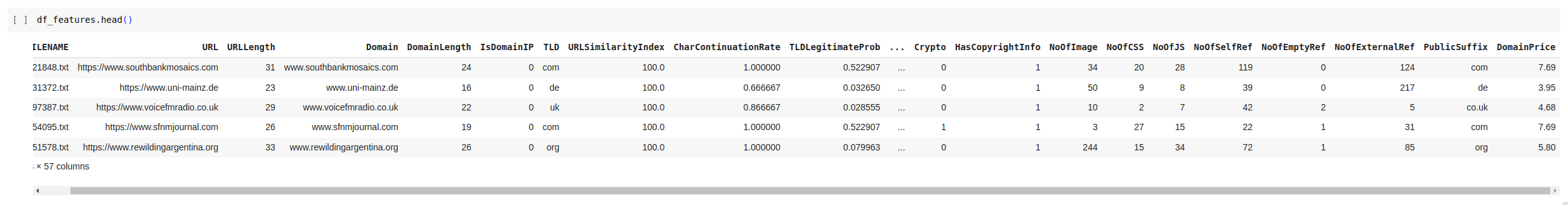
Remove Unnecessary Labels
We will remove the columns that are not needed for the analysis. This includes the Title, URL, Domain, and FILENAME columns.
NOTE: These columns are not needed for the analysis but could be useful for other types of analysis such as NLP or extracting additional features if needed.
df_features = df_features.drop(columns=['Title', 'URL', 'Domain', 'FILENAME'])Understanding Features (Input) Data
## sort the columns in alphabetic order
df_features = df_features.reindex(sorted(df_features.columns), axis=1).reset_index(drop=True)

df_features.nunique() # number of unique values
Output:
Bank                               2
CharContinuationRate             898
Crypto                             2
DegitRatioInURL                  575
DomainLength                     101
DomainPrice                      406
DomainTitleMatchScore            152
HasCopyrightInfo                   2
HasDescription                     2
HasExternalFormSubmit              2
HasFavicon                         2
HasHiddenFields                    2
HasObfuscation                     2
HasPasswordField                   2
HasSocialNet                       2
HasSubmitButton                    2
HasTitle                           2
IsDomainIP                         2
IsHTTPS                            2
IsResponsive                       2
LargestLineLength              26181
LetterRatioInURL                 709
LineOfCode                     10738
NoOfAmpersandInURL                31
NoOfCSS                          209
NoOfDegitsInURL                  182
NoOfEmptyRef                     296
NoOfEqualsInURL                   25
NoOfExternalRef                 1191
NoOfImage                        992
NoOfJS                           253
NoOfLettersInURL                 421
NoOfObfuscatedChar                20
NoOfOtherSpecialCharsInURL        74
NoOfPopup                        115
NoOfQMarkInURL                     5
NoOfSelfRedirect                   2
NoOfSelfRef                     1374
NoOfSubDomain                     10
NoOfURLRedirect                    2
NoOfiFrame                       119
ObfuscationRatio                 146
Pay                                2
PublicSuffix                    2100
Robots                             2
SpacialCharRatioInURL            240
TLD                              570
TLDLegitimateProb                465
TLDLength                         12
URLCharProb                   227421
URLLength                        482
URLSimilarityIndex             36360
URLTitleMatchScore               497
dtype: int64
Note that although many fields appear numerical, they could actually be categorical, especially if some fields have only 2 unique values.
Additionally, labels with names beginning with "Has" or "Is" are likely to be categorical data.
df_features.describe()

print(f"Number of total features: {df_features.shape[1]}, before splitting")
Number of total features: 53, before splitting.
Split numerical and categorical input features
## split non-numeric and numeric columns
df_features_numerical = df_features.select_dtypes(include=[np.number])
df_features_categorical = df_features.select_dtypes(exclude=[np.number])

## categorize the columns with field name starting with 'Has' and 'Is' as categorical
has_columns = [col for col in df_features.columns if col.startswith('Has')]
is_columns = [col for col in df_features.columns if col.startswith('Is')]

df_features_categorical = pd.concat([df_features_categorical, df_features[has_columns], df_features[is_columns]], axis=1)
df_features_numerical = df_features_numerical.drop(columns=has_columns + is_columns)

df_features_numerical.describe() # to examine if they are indeed numerical
Let’s move while observing the features to categorical if they only have 0 and 1 values.
## move the features to categorical if they only have 0 and 1 values
for col in df_features_numerical.columns:
    if df_features_numerical[col].nunique() == 2:
        if set(df_features_numerical[col].unique()) == {0, 1}:
            print(f"Moving {col} to categorical")
            df_features_categorical[col] = df_features_numerical[col]
            df_features_numerical = df_features_numerical.drop(columns=col)
Output (checked the values to make sure they are indeed categorical):
Moving Bank to categorical
Moving Crypto to categorical
Moving NoOfSelfRedirect to categorical
Moving NoOfURLRedirect to categorical
Moving Pay to categorical
Moving Robots to categorical
After splitting the data:
print(f"Number of numerical features: {df_features_numerical.shape[1]}")
print(f"Number of categorical features: {df_features_categorical.shape[1]}")
print(f"Total number of features: {df_features_numerical.shape[1] + df_features_categorical.shape[1]}")
We have identified:
- 32 numerical features
- 21 categorical features
- A total of 53 features
df_features_numerical.dtypes
df_features_numerical.nunique() # number of unique values

df_features_categorical.dtypes
df_features_categorical.nunique() # number of unique values
## Field names of categorical data:
df_features_categorical.columns
Index(['PublicSuffix', 'TLD', 'HasCopyrightInfo', 'HasDescription',
'HasExternalFormSubmit', 'HasFavicon', 'HasHiddenFields',
'HasObfuscation', 'HasPasswordField', 'HasSocialNet', 'HasSubmitButton',
'HasTitle', 'IsDomainIP', 'IsHTTPS', 'IsResponsive', 'Bank', 'Crypto',
'NoOfSelfRedirect', 'NoOfURLRedirect', 'Pay', 'Robots'],
dtype='object')
## Field names of numerical data:
df_features_numerical.columns
Index(['CharContinuationRate', 'DegitRatioInURL', 'DomainLength',
'DomainPrice', 'DomainTitleMatchScore', 'LargestLineLength',
'LetterRatioInURL', 'LineOfCode', 'NoOfAmpersandInURL', 'NoOfCSS',
'NoOfDegitsInURL', 'NoOfEmptyRef', 'NoOfEqualsInURL', 'NoOfExternalRef',
'NoOfImage', 'NoOfJS', 'NoOfLettersInURL', 'NoOfObfuscatedChar',
'NoOfOtherSpecialCharsInURL', 'NoOfPopup', 'NoOfQMarkInURL',
'NoOfSelfRef', 'NoOfSubDomain', 'NoOfiFrame', 'ObfuscationRatio',
'SpacialCharRatioInURL', 'TLDLegitimateProb', 'TLDLength',
'URLCharProb', 'URLLength', 'URLSimilarityIndex', 'URLTitleMatchScore'],
dtype='object')We will proceed to analyze the data following the split.
One Hot Encoding
In machine learning, most algorithms require input data in a numerical format because they perform calculations with these numbers during the learning process. Categorical data, such as labels or categories, inherently lack a numerical representation and thus cannot be directly processed by these algorithms.
Converting these categorical variables into a numerical format allows machine learning algorithms to efficiently include these features in computations for tasks like classification or regression.
Let’s now convert our categorical variables from two DataFrame subsets (df_features_categorical and df_features) into numerical format by applying one-hot encoding.
## One hot encode categorical labels
if do_one_hot_encoding:
    df_features_categorical_encoded = pd.get_dummies(df_features_categorical, columns=categorical_columns_lst)
    df_features_encoded = pd.get_dummies(df_features, columns=categorical_columns_lst)
Completing the Preprocessing Steps
We have successfully completed the data preprocessing steps and now have the following dataframes ready for our next steps:
df_urls_datacontains the original dataset, including both features and target.df_featurescontains the features only.df_features_rawcontains the raw features such as the URL, Title, and Domain.df_features_encodedcontains the encoded features.df_targetcontains the target only.df_features_numericalcontains the numerical features only.df_features_categoricalcontains the categorical features only.df_features_categorical_encodedcontains the encoded categorical features
Exploratory Data Analysis
Install Dependencies
First, let's install the required dependencies and then import them.
!pip install pandas numpy matplotlib seaborn scikit-learn

## visualization of missing values
!pip install missingno

## plotly
!pip install plotly
!pip install "nbformat>=4.2.0"

## country codes conversion
!pip install pycountry

## scipy
!pip install scipy
## import packages
import pandas as pd
import numpy as np
import missingno as msno
from scipy.stats import chi2_contingency
from scipy.stats import ttest_ind
import matplotlib.pyplot as plt
import seaborn as sns
from collections import Counter
import seaborn as sns
import plotly.express as px## Check the first 5 rows to get a feel of the data
df_urls_data.head()
Let's also check the shape of the dataframes. Make sure they are loaded correctly from the preprocessing notebook.
## Check the shape of categorical data
print(f"Shape of df_features_categorical: {df_features_categorical.shape}")
print("Data types of df_features:")
df_features_categorical.info()

## Check the shape of numerical data
print(f"Shape of df_features_numerical: {df_features_numerical.shape}")
print("Data types of df_features_numerical:")
df_features_numerical.info()
Shape of df_features_categorical: (235795, 21)
Data types of df_features:
<class 'pandas.core.frame.DataFrame'>
RangeIndex: 235795 entries, 0 to 235794
Data columns (total 21 columns):
# Column Non-Null Count Dtype
--- ------ -------------- -----
0 PublicSuffix 235795 non-null object
1 TLD 235795 non-null object
2 HasCopyrightInfo 235795 non-null int64
3 HasDescription 235795 non-null int64
4 HasExternalFormSubmit 235795 non-null int64
5 HasFavicon 235795 non-null int64
6 HasHiddenFields 235795 non-null int64
7 HasObfuscation 235795 non-null int64
8 HasPasswordField 235795 non-null int64
9 HasSocialNet 235795 non-null int64
10 HasSubmitButton 235795 non-null int64
11 HasTitle 235795 non-null int64
12 IsDomainIP 235795 non-null int64
13 IsHTTPS 235795 non-null int64
14 IsResponsive 235795 non-null int64
15 Bank 235795 non-null int64
16 Crypto 235795 non-null int64
17 NoOfSelfRedirect 235795 non-null int64
18 NoOfURLRedirect 235795 non-null int64
19 Pay 235795 non-null int64
20 Robots 235795 non-null int64
dtypes: int64(19), object(2)
memory usage: 37.8+ MB
Shape of df_features_numerical: (235795, 32)
Data types of df_features_numerical:
<class 'pandas.core.frame.DataFrame'>
RangeIndex: 235795 entries, 0 to 235794
Data columns (total 32 columns):
# Column Non-Null Count Dtype
--- ------ -------------- -----
0 CharContinuationRate 235795 non-null float64
1 DegitRatioInURL 235795 non-null float64
2 DomainLength 235795 non-null int64
3 DomainPrice 235795 non-null float64
4 DomainTitleMatchScore 235795 non-null float64
5 LargestLineLength 235795 non-null int64
6 LetterRatioInURL 235795 non-null float64
7 LineOfCode 235795 non-null int64
8 NoOfAmpersandInURL 235795 non-null int64
9 NoOfCSS 235795 non-null int64
10 NoOfDegitsInURL 235795 non-null int64
11 NoOfEmptyRef 235795 non-null int64
12 NoOfEqualsInURL 235795 non-null int64
13 NoOfExternalRef 235795 non-null int64
14 NoOfImage 235795 non-null int64
15 NoOfJS 235795 non-null int64
16 NoOfLettersInURL 235795 non-null int64
17 NoOfObfuscatedChar 235795 non-null int64
18 NoOfOtherSpecialCharsInURL 235795 non-null int64
19 NoOfPopup 235795 non-null int64
20 NoOfQMarkInURL 235795 non-null int64
21 NoOfSelfRef 235795 non-null int64
22 NoOfSubDomain 235795 non-null int64
23 NoOfiFrame 235795 non-null int64
24 ObfuscationRatio 235795 non-null float64
25 SpacialCharRatioInURL 235795 non-null float64
26 TLDLegitimateProb 235795 non-null float64
27 TLDLength 235795 non-null int64
28 URLCharProb 235795 non-null float64
29 URLLength 235795 non-null int64
30 URLSimilarityIndex 235795 non-null float64
31 URLTitleMatchScore 235795 non-null float64
dtypes: float64(11), int64(21)
memory usage: 57.6 MB## Visualize missing values as a matrix
msno.matrix(df_features_categorical)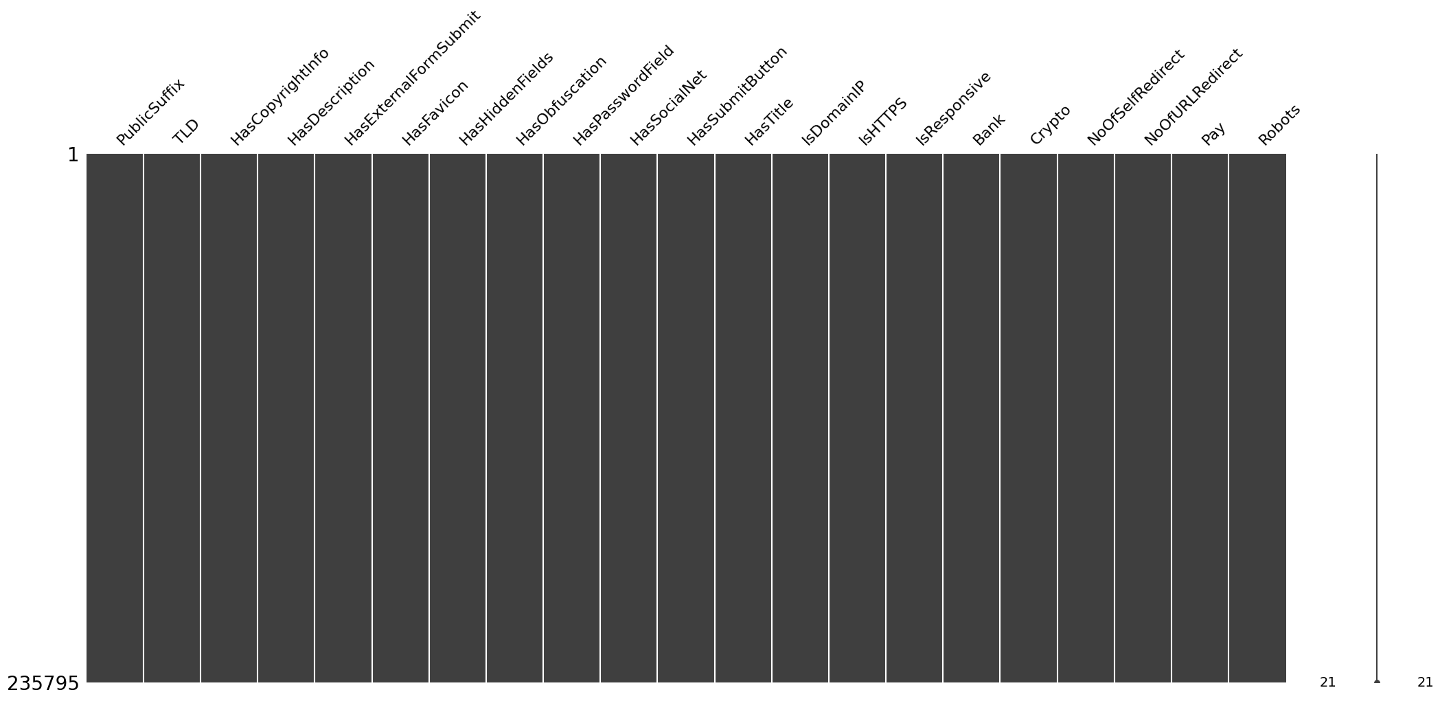
It appears that there are no missing values in the dataset. This is good news!
Understanding Target Data
Number of phishing vs legitimate data
The target label of this dataset is binary, where 0 represents phishing and 1 represents legitimate.
So, the next question come to my mind: How balanced is the target of our dataset?
Check how many phishing and non-phishing data in the dataset.
non_phishing_counts = sum(df_target['label'] == 1)
phishing_counts = sum(df_target['label'] == 0)

## let's count the number of phishing and non-phishing URLs
print(f"Non-phishing counts: {non_phishing_counts} "
      f"(Percentage: {non_phishing_counts/len(df_target)*100:.2f}%)") #get percentage
print(f"Phishing counts: {phishing_counts} "
      f"(Percentage: {phishing_counts/len(df_target)*100:.2f}%)") #get percentage
We obtained:
- Non-phishing counts: 134850 (Percentage: 57.19%)
- Phishing counts: 100945 (Percentage: 42.81%)
Let's also visualize the distribution of the target label.
plt.figure(figsize=(6, 4))

## Plot for phishing
sns.countplot(x='label',
data=df_target, hue='label',
palette='viridis')

plt.title('Count of Phishing vs Non-Phishing URLs')
plt.xlabel('label')
plt.ylabel('Count')
plt.xticks(ticks=[0, 1],
            labels=['Phishing','Non-Phishing'])

plt.show()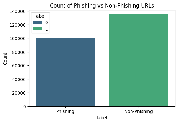
Based on the distribution, we can see the target label is not too imbalanced. We can proceed with the dataset as it is.
Understanding Numerical Features
Correlation Matrix
## combine df_features_numerical and df_target
df_urls_numerical = pd.concat([df_features_numerical, df_target], axis=1)

columns = df_urls_numerical.columns.tolist()

corr_mat = df_urls_numerical.corr()

plt.figure(figsize=(64, 64))
sns.heatmap(
    corr_mat,
    cmap='RdBu',
    vmin=-1,
    vmax=1,
    center=0,
    annot=True,
    fmt=".1f"
)

plt.show()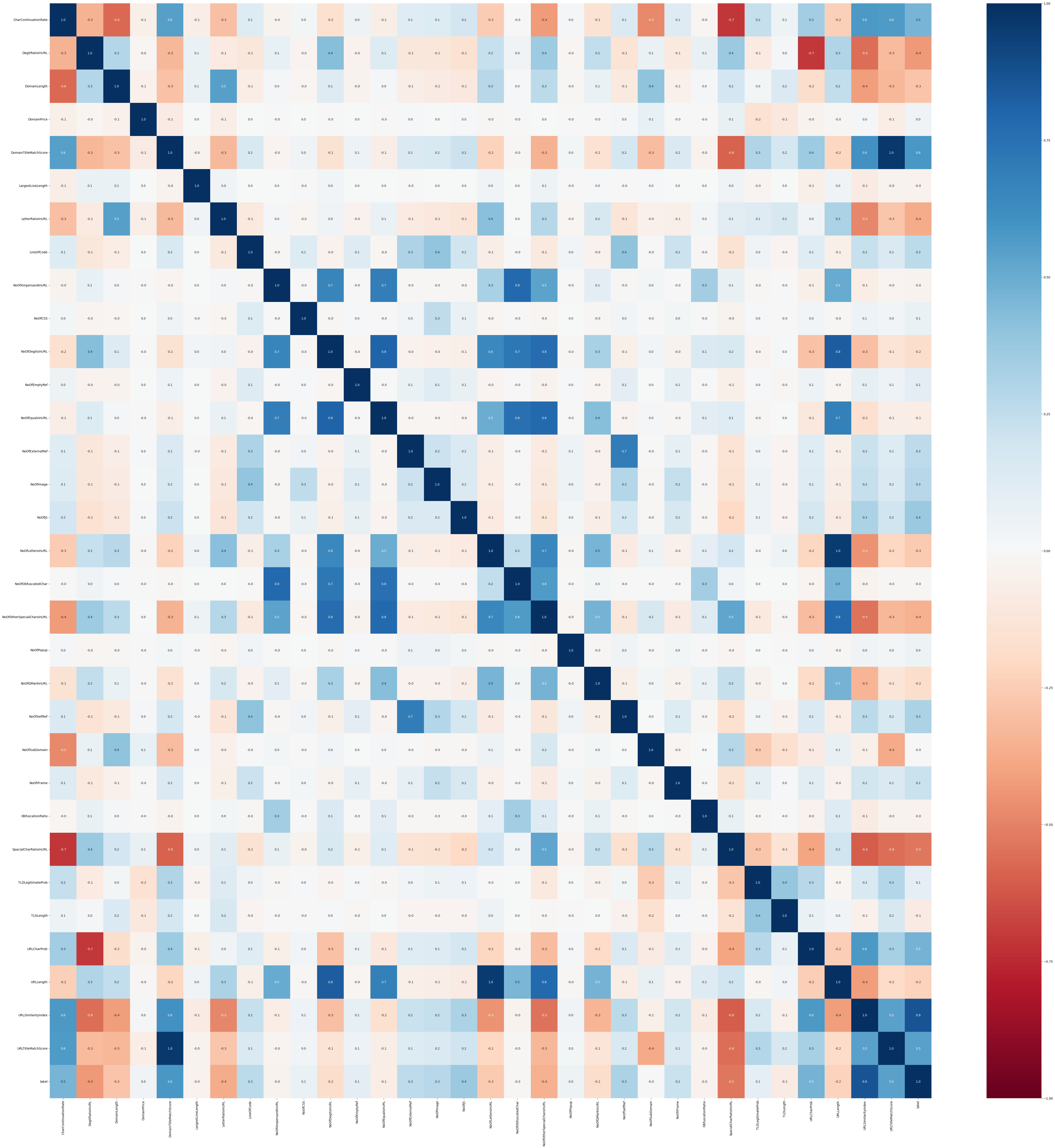
Identify the feature pairs that have high correlation (threshold = 0.8):
- NoOfEqualsInURL and NoOfDegitsInURL has high correlation = 0.80602442162387
- URLLength and NoOfDegitsInURL has high correlation = 0.8358093990245989
- URLLength and NoOfLettersInURL has high correlation = 0.9560469859044239
- URLTitleMatchScore and DomainTitleMatchScore has high correlation = 0.9610084343550412
- label and URLSimilarityIndex has high correlation = 0.8603580349950561
## Print features having high correlation with the target 'label'
corr_target = corr_mat['label'].sort_values(ascending=False)
corr_target_top_5 = corr_target.head(6)
corr_target_top_5 = corr_target_top_5[1:] # remove label itself

corr_target_top_5
URLSimilarityIndex 0.860358
DomainTitleMatchScore 0.584905
URLTitleMatchScore 0.539419
URLCharProb 0.469749
CharContinuationRate 0.467735
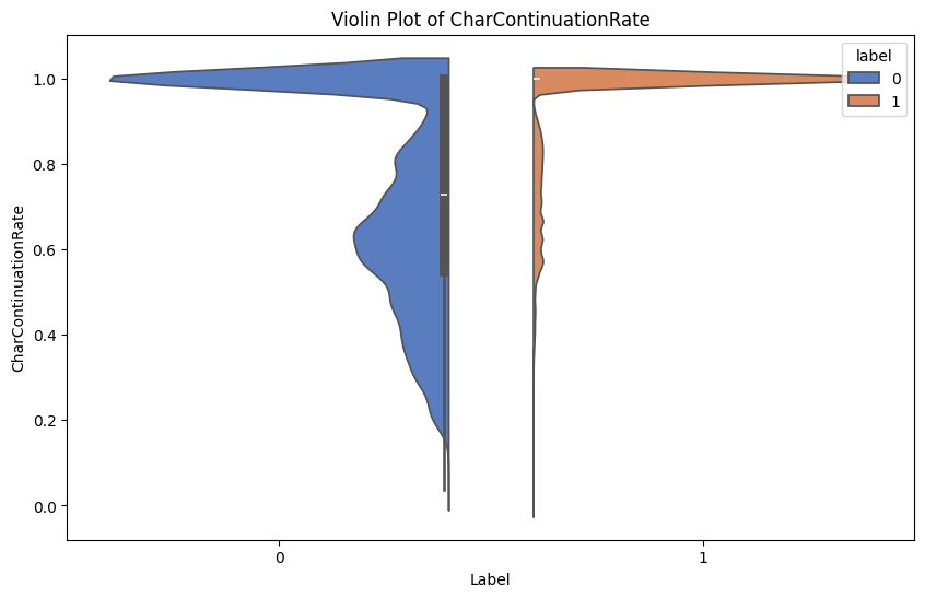
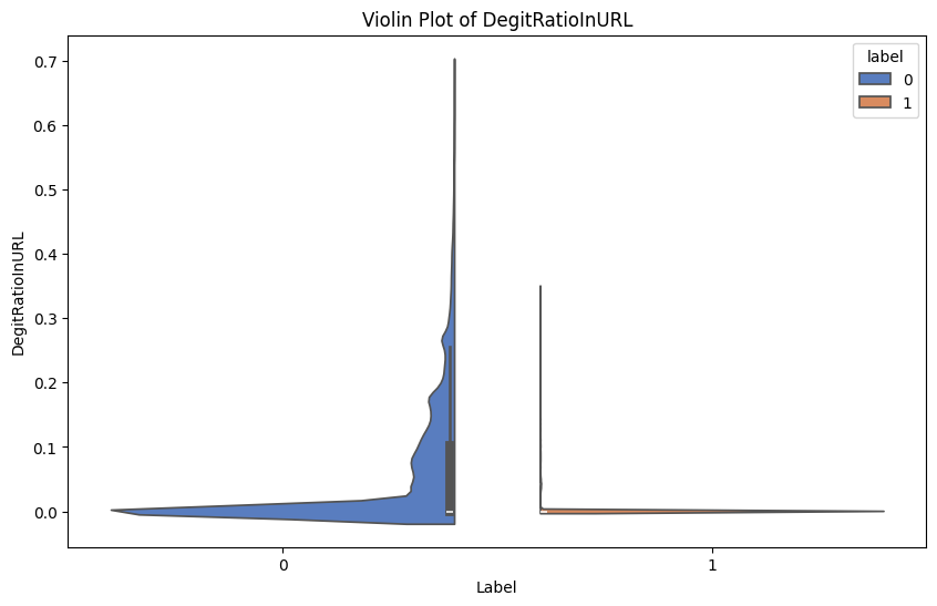
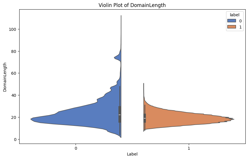
Name: label, dtype: float64Violin Plots
Plot violin plots for the numerical features with the target label Phishing.
Recall 0 represents phishing and 1 represents legitimate.
for feature in columns:
    plt.figure(figsize=(10, 6))
    sns.violinplot(x='label', y=feature, data=df_urls_numerical, hue='label', split=True, palette='muted')
    plt.title(f'Violin Plot of {feature}')
    plt.xlabel('Label')
    plt.ylabel(feature)
    plt.show()
Here are some examples of the generated violin plots:
Interactive Box Plots
Plot for the top 5 features that have the highest correlation with the target.
NOTE: To view the interactive plot, you MUST run the code below. The plot is not saved as an image in the notebook, so you won't be able to see it if you don't run the code.
for column in corr_target_top_5.index:
    fig = px.box(df_urls_numerical, y=column, color=df_target['label'])
    fig.show()
Statistical Tests
For all numerical features, perform t-tests to compare means:
numerical_t_results = {}

for feature in columns:
    # skip label
    if feature == 'label':
        continue
    phishing = df_features_numerical[df_target['label'] == 0][feature]
    non_phishing = df_features_numerical[df_target['label'] == 1][feature]
    t_stat, p_val = ttest_ind(phishing, non_phishing)
    print(f"T-test for {feature}: Stat={t_stat}, P-value={p_val}")
    numerical_t_results[feature] = (t_stat, p_val)
Most Important Numerical Features
Features with small p-values are considered more important for our classification model.
## top features with the smallest p-value
numerical_t_results_sorted = sorted(numerical_t_results.items(), key=lambda x: x[1][1])
numerical_t_results_sorted[:10]
That gives us
[('CharContinuationRate', (-256.9673224005409, 0.0)),
 ('DegitRatioInURL', (232.61796808324493, 0.0)),
 ('DomainLength', (143.36142600843974, 0.0)),
 ('DomainTitleMatchScore', (-350.1667834107168, 0.0)),
 ('LetterRatioInURL', (192.05733596392525, 0.0)),
 ('LineOfCode', (-137.3940419972396, 0.0)),
 ('NoOfDegitsInURL', (87.82689697158546, 0.0)),
 ('NoOfEmptyRef', (-53.36214828900374, 0.0)),
 ('NoOfExternalRef', (-130.00859090242156, 0.0)),
('NoOfImage', (-138.7039740466059, 0.0))]-
SpacialCharRatioInURL,DegitRatioInURL,LetterRatioInURL,NoOfOtherSpecialCharsInURL:This aligns with my personal experience that phishing URLs frequently use special characters, digits, and unusual letter combinations to mimic legitimate URLs, or to create confusing URLs that are more likely to deceive users.
-
DomainLength,NoOfLettersInURL,URLLength:These features being important makes sense because longer URLs are often used by phishers to hide malicious subdomains or paths that resemble legitimate addresses.
-
NoOfDegitsInURL,NoOfQMarkInURL:Phishing URLs may contain some digits in the url to resemble legitimate URLs. For example, if phishers want to peform phishing against UPenn students, the
upenn.edudomain is appearently already registered, so they may registerupenn1[.]comorupenn2024[.]educationto trick users. -
TLDLength:Abnormal TLD lengths can indicate less common or exotic TLDs used by phishers to create credible-looking URLs, for example,
upenn-pay[.]comorupenn-login[.]education.
Weakest Numerical Features
These are the features that have the weakest statistical significance.
## top 5 features with the largest p-value
numerical_t_results_sorted[-5:]
That gives us
[('DomainPrice', (-20.15339051241565, 2.9952761186943435e-90)),
 ('LargestLineLength', (19.979571665743187, 9.826104450198757e-89)),
 ('NoOfAmpersandInURL', (16.821978666871274, 1.834605816231233e-63)),
 ('NoOfObfuscatedChar', (7.437398819558432, 1.0303278198240061e-13)),
 ('NoOfSubDomain', (2.8917740201365536, 0.0038310837128889526))]
Understanding Categorical Features
## combine df_features_categorical and df_target
df_urls_categorical_visual = pd.concat([df_features_categorical, df_target], axis=1).copy()
For the categorical labels, let's visualize the distribution of the features against the target label.
What are we looking for here? We are looking for features that have a significant difference between counts of phishing and non-phishing URLs. If one has very distinct difference, this feature could play a significant role in impacting the target label.
## descriptive text for the label
df_urls_categorical_visual['label_text'] = df_urls_categorical_visual['label'].map({0: 'Non-Phishing', 1: 'Phishing'})

## Skip columns with too many unique values,
##for example urls here is not useful for direct comparison
skipped_column_names = ['TLD', 'PublicSuffix', 'label', 'label_text']

for column in df_urls_categorical_visual.columns:
    if column not in skipped_column_names:
        plt.figure(figsize=(10, 4))
        ax = sns.countplot(data=df_urls_categorical_visual, x=column, hue="label_text", palette="Set1")
        plt.title(f'Distribution of {column}')
        plt.xticks(rotation=45)
        plt.legend(title='Label', loc='upper right', bbox_to_anchor=(1.05, 1), borderaxespad=0.)
        plt.show()
Statistical Testing for Categorical Features
The visualization above is useful to get a feeling of the distribution of the categorical features and their significance in relationship with the target label.
Now, let's perform statistical tests to confirm the significance of the features.
Here we use Chi-test, which is primarily used to examine whether two categorical variables (two dimensions of the contingency table) are independent in influencing the test statistic (values within the table)
Mathematically, a Chi-Square test is done on two distributions two determine the level of similarity of their respective variances. In its null hypothesis, it assumes that the given distributions are independent. This test thus can be used to determine the best features for a given dataset by determining the features on which the output class label is most dependent. For each feature in the dataset, the $\chi ^{2}$ is calculated and then ordered in descending order according to the $\chi ^{2}$ value. The higher the value of $\chi ^{2}$ , the more dependent the output label is on the feature and higher the importance the feature has on determining the output. Let the feature in question have m attribute values and the output have k class labels. Then the value of $\chi ^{2}$ is given by the following expression:
$\chi ^{2} = \sum {i=1}^{m} \sum {j=1}^{k}\frac{(O{ij}-E{ij})^{2}}{E_{ij}}$
where $O{ij}$ – Observed frequency $E{ij}$ – Expected frequency For each feature, a contingency table is created with m rows and k columns. Each cell (i,j) denotes the number of rows having attribute feature as i and class label as k. Thus each cell in this table denotes the observed frequency. (source)
def perform_chi2_test(df, feature):
    contingency_table = pd.crosstab(df[feature], df['label'])
    chi2, p, dof, expected = chi2_contingency(contingency_table)
    print(f"Chi-squared test for {feature}:")
    print(f"Chi2 Statistic: {chi2}, P-value: {p}\n")
    return chi2, p

chi2_stats = {}

## Perform test for each categorical feature
for column in df_urls_categorical_visual.columns:
    if column not in ['label', 'label_text']:
        chi2,p = perform_chi2_test(df_urls_categorical_visual, column)
        chi2_stats[column] = (chi2, p)
To help us better understand the importance, let's rank them by their $\chi ^{2}$ values.
## Order by significance
chi2_stats_sorted = sorted(chi2_stats.items(), key=lambda x: x[1][0], reverse=True)
chi2_stats_sorted
[('HasSocialNet', (145023.7420316948, 0.0)),
('HasCopyrightInfo', (130292.68757967741, 0.0)),
('HasDescription', (112334.62388393158, 0.0)),
('PublicSuffix', (90887.69233733535, 0.0)),
('IsHTTPS', (87486.78604118452, 0.0)),
('HasSubmitButton', (78925.93676851525, 0.0)),
('TLD', (72390.61558625728, 0.0)),
('IsResponsive', (70964.98848503799, 0.0)),
('HasHiddenFields', (60783.768711655066, 0.0)),
('HasFavicon', (57473.0059661682, 0.0)),
('HasTitle', (49831.82697877125, 0.0)),
('Robots', (36346.1017555631, 0.0)),
('Pay', (30514.30996266347, 0.0)),
('Bank', (8418.032312347743, 0.0)),
('HasExternalFormSubmit', (6619.679733768652, 0.0)),
('HasPasswordField', (4501.468438718974, 0.0)),
('Crypto', (2338.26408286789, 0.0)),
('NoOfSelfRedirect', (1377.8103615413584, 1.3941584604567876e-301)),
('IsDomainIP', (852.260590396482, 2.3448225852057846e-187)),
('HasObfuscation', (646.896659124284, 1.0568883774203827e-142)),
('NoOfURLRedirect', (508.61027713202554, 1.2722702420876379e-112))]The Chi-Square test results show that the top features that have the highest $\chi ^{2}$ values are:
-
HasSocialNet(Chi2 Statistic: 145023.7420316948, P-value: 0.0):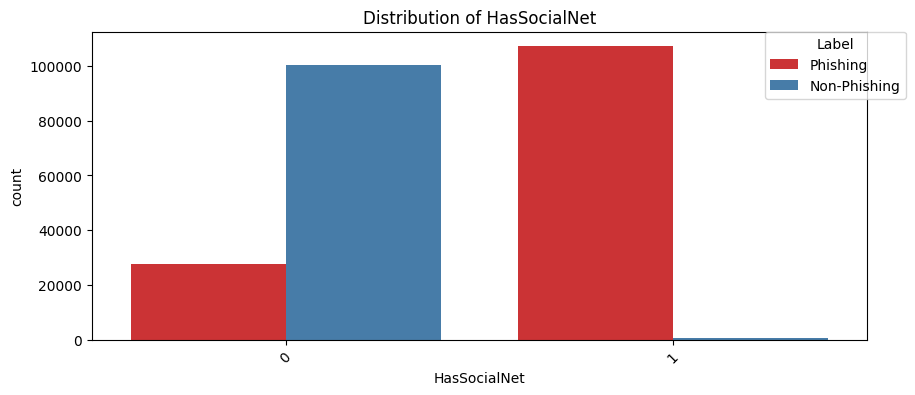
This feature shows us whether a website includes social network links, which is typical for legitimate sites as they often connect to many social media platforms for marketing purposes. For example, we know that UPenn's website https://www.upenn.edu typically has links to their Facebook, Twitter, and Instagram pages, etc. The phishign sites, as you may expect, are less likely to include these links, as most of them are not interested in promoting their site on social media.
-
HasCopyrightInfo(Chi2 Statistic: 130292.68757967741, P-value: 0.0):
Copyright information adds legitimacy to a website by indicating ownership and the legality of content, which is another common indication of a legitimate site.
For example, UPenn's website https://www.upenn.edu has the following copyright information in the footer:
<p style="text-align: center;"><strong><a href="<https://www.seas.upenn.edu/>">
   PENN ENGINEERING </a>©2017</strong>
</p>
Phishing sites woudn't bother adding these info on their website.
-
HasDescription(Chi2 Statistic: 112334.62388393158, P-value: 0.0):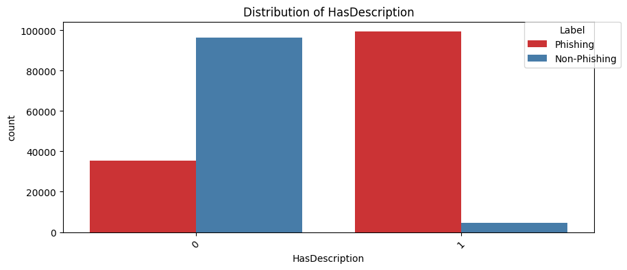
Meta descriptions in the headers usually, if SEO is done right, provide a summary of the website's content on search engine results.
For example, https://www.seas.upenn.edu has the following meta description in the header:
<meta name="description" content="Penn Engineering | Inventing the Future">Again, a phishing site wouldn't bother with SEO aspect of things on their websites.
-
HasSubmitButton(Chi2 Statistic: 78925.93676851525, P-value: 0.0):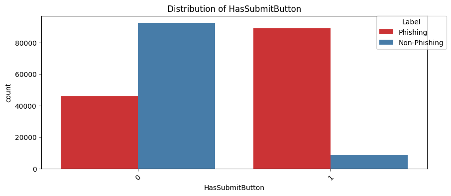
The presence of a submit button is common in forms where user input is required. Legitimate sites design these elements to be user-friendly and secure. Phishing sites often have forms designed to harvest data, so there is a higher chance of them having submit buttons.
-
IsHTTPS(Chi2 Statistic: 87486.78604118452, P-value: 0.0):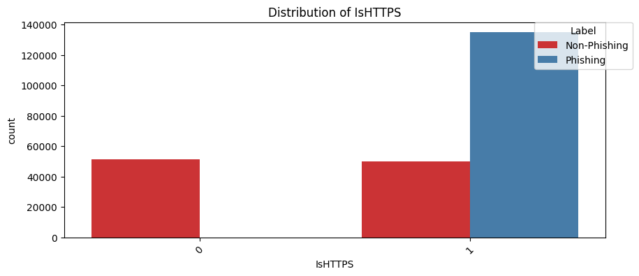
HTTPS indicates that a site uses a secure protocol with installed SSL cert to encrypt data between the user and the server. Many phishing sites now also use HTTPS to appear legitimate, at least for those ones I personally encountered. The significant chi-squared statistic shows this feature is statistically significant for distinguishing between phishing and non-phishing sites.
-
HasFavicon(Chi2 Statistic: 57473.0059661682, P-value: 0.0):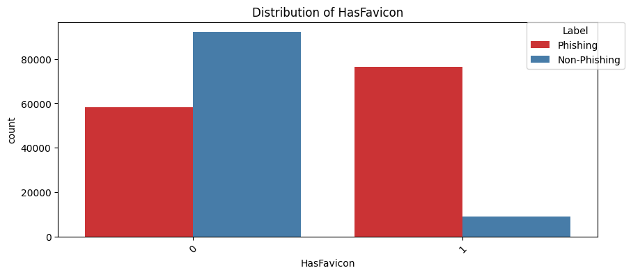
Favicons are small icons associated with a website, typically displayed in browser tabs and bookmarks. For example, visiting UPenn website https://www.upenn.edu will show you the UPenn logo in the browser tab. Phishing sites might not use custom favicons.
TLD Phishing Abuse Analysis over the TLD field
Top-level domains (TLDs), which are the final segments of a domain name, are frequently utilized by malicious actors. They often create domains with TLDs that mimic well-known and trusted extensions, deceiving users into visiting counterfeit websites (Anon, 2023a).
The introduction of new TLDs like .zip and .mov has enabled cybercriminals to register domains that look like familiar file extensions. This can mislead users into thinking they are downloading a safe file, when in fact, they are being directed to a phishing URL.
Shortly after the release of these TLDs, numerous phishing domains were registered (Anon, 2023b). Phishers commonly use TLDs that mirror well-known brands or trusted entities to trick users into believing they are accessing legitimate websites. (source)
So, let's analyze the TLD field to see if there are any patterns that we can identify.
## List the top 20 most frequentlt abused TLDs
df_urls_categorical_phishing = df_urls_categorical_visual[df_urls_categorical_visual['label'] == 0] # 0 is phishing
top_phishing_tlds = df_urls_categorical_phishing['TLD'].value_counts().head(50)
## top_phishing_tlds
## histogram for top_phishing_tlds
plt.figure(figsize=(10, 6))
sns.barplot(x=top_phishing_tlds.index, y=top_phishing_tlds.values, legend=False)
plt.title('Top 50 Most Frequently Abused TLDs')
plt.xlabel('Top Level Domains')
plt.ylabel('Count')
plt.xticks(rotation=90)
plt.show()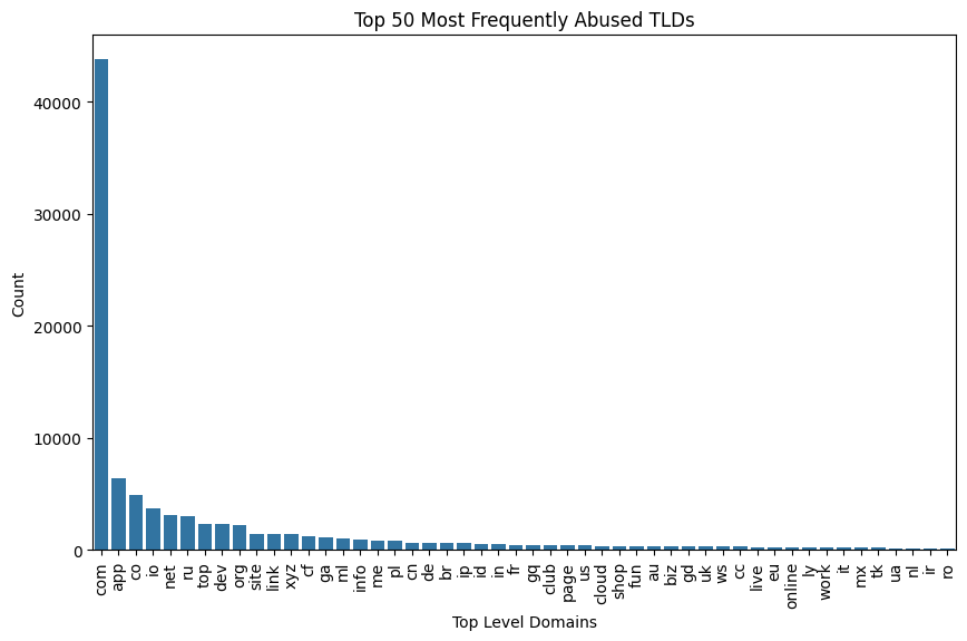
The Most Abused ccTLDs (country code TLDs)
ccTLD is a top-level domain that is generally reserved or used for a country or a dependent territory.
For example, .us is the ccTLD for the United States. The ccTLDs are assigned by the Internet Assigned Numbers Authority (IANA) to the national governments of countries and are always two letters long.
For more info about ccTLD: https://icannwiki.org/Country_code_top-level_domain
So, let's filter for the domains that have ccTLDs.
## Filter for only ccTLDs (2 chars) from TLDs
df_urls_categorical_cctlds = df_urls_categorical_visual[df_urls_categorical_visual['TLD'].str.len() == 2]
print(f"Number of ccTLDs: {len(df_urls_categorical_cctlds)}")
## Number of ccTLDs: 69596

## List the top 20 most frequently abused ccTLDs
df_urls_categorical_phishing_cctlds = df_urls_categorical_cctlds[df_urls_categorical_cctlds['label'] == 0] # 0 is phishing
top_phishing_cctlds = df_urls_categorical_phishing_cctlds['TLD'].value_counts().head(50)
top_phishing_cctlds

##get a list of countries and a list of counts
abused_cctld_countries = top_phishing_cctlds.index.tolist()
abused_cctld_counts = top_phishing_cctlds.values.tolist()
## histogram for top_phishing_cctlds
plt.figure(figsize=(10, 6))
sns.barplot(x=top_phishing_cctlds.index, y=top_phishing_cctlds.values, legend=False)
plt.title('Top 50 Most Frequently Abused ccTLDs')
plt.xlabel('Country Top Level Domains')
plt.ylabel('Count')
plt.xticks(rotation=90)
plt.show()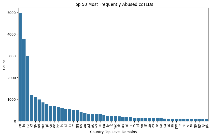
Global Heat Map of ccTLD Phishing Abuse Counts
Finally, let's visualize the global distribution of the ccTLD abuse counts on a world map.
Because the plotly package supports only 3 letter country codes, we need to map the 2 letter country codes to 3 letter country codes using the pycountry package.
import pycountry

## convet two-letter codes to three-letter ISO codes
def alpha2_to_alpha3(alpha2):
    country = pycountry.countries.get(alpha_2=alpha2.upper())
    print(f"Country: {country}")
    return country.alpha_3 if country else None
Plot a global map based on the two digit country codes:
## Create a DataFrame for plotting
data = pd.DataFrame({
    'Country': [alpha2_to_alpha3(cc)
                for cc in abused_cctld_countries],
    'Counts': abused_cctld_counts
})

## Plot a global map based on the two digit country codes
fig = px.choropleth(
    data_frame=data,
    locations='Country',
    locationmode='ISO-3',
    color='Counts',
    title='Global Map of Most Abused ccTLDs',
    hover_name='Country',
    color_continuous_scale=px.colors.sequential.Bluered,
    projection='natural earth'
)

fig.show()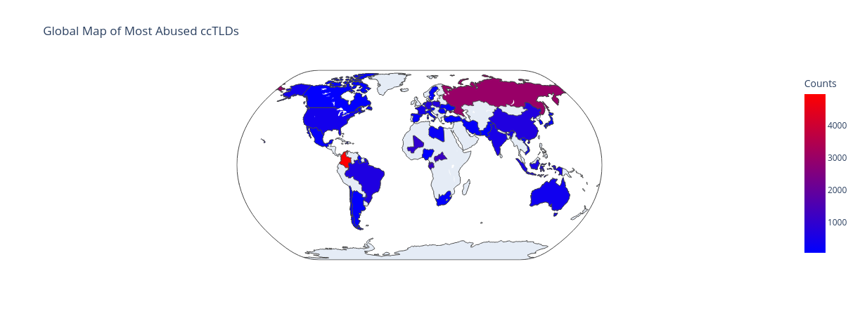
The following bullet list provides a brief overview of some of the most abused country code top-level domains (ccTLDs):
- Colombia (.co): 4964 instances
- British Indian Ocean Territory (.io): 3769 instances
- Russia (.ru): 2983 instances
- Central African Republic (.cf): 1203 instances
- Gabon (.ga): 1107 instances
- Mali (.ml): 994 instances
- Montenegro (.me): 853 instances
- Poland (.pl): 802 instances
- China (.cn): 690 instances
- Germany (.de): 686 instances
- Brazil (.br): 653 instances
- Philippines (.ph): 608 instances
- Indonesia (.id): 560 instances
- India (.in): 537 instances
Logistic Regression
In this analysis, we first use the basic Logistic Regression for binary classification task.
lr = LogisticRegression()
lr.fit(X_train, y_train)

## Use the model to predict on the test set and save these predictions as `y_pred`
y_pred = lr.predict(X_test)

## Find the accuracy and store the value in `log_acc`
log_acc = lr.score(X_test, y_test)

print(f"accuracy: {log_acc}")

## accuracy: 0.9971302958763907
The accuracy of the Logistic Regression model, as determined by comparing the predicted labels against the actual labels in y_test, is impressively high at approximately 99.71%.
PCA to Reduce Dimensionality
Before proceeding with another round of Logistic Regression, we apply Principal Component Analysis (PCA) to reduce the dimensionality of the feature set. PCA is a statistical technique that transforms a large set of variables into a smaller one that still contains most of the information in the large set.
First, the feature set is standardized to ensure that PCA's performance is not biased by the nature of scale invariance.
std_s = StandardScaler()
X_train_scaler = std_s.fit_transform(X_train)
X_test_scaler = std_s.transform(X_test)

## Instantiate and Fit PCA
pca = PCA(n_components = X_train_scaler.shape[1])
pca_x_train = pca.fit_transform(X_train_scaler)

## Save the explained variance ratios
explained_variance_ratios = pca.explained_variance_ratio_

## Save the CUMULATIVE explained variance ratios
cum_evr = np.cumsum(explained_variance_ratios)
By examining the cumulative explained variance ratio, we determine the number of components that account for 80% of the variance in the dataset:
thresh = 0.8

## Plotting
plt.figure(figsize=(8, 6))
sns.lineplot(x=np.arange(1, len(cum_evr) + 1), y=cum_evr, label='Cumulative Explained Variance')
sns.lineplot(x=np.arange(1, len(cum_evr) + 1), y=[thresh] * len(cum_evr), linestyle='--', label='80% Threshold')

plt.xlabel('Number of Components')
plt.ylabel('Cumulative Explained Variance Ratio')
plt.title('Cumulative Explained Variance Ratio vs. Number of Components')
plt.xticks(ticks=np.arange(1, len(explained_variance_ratios) + 1, step=max(1, len(explained_variance_ratios) // 10)))  # Adjust step for readability
plt.legend()
plt.show()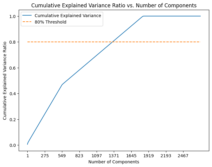
pca = PCA(n_components = num_components)
X_train_pca = pca.fit_transform(X_train_scaler)

## Transform on Testing Set
X_test_pca = pca.transform(X_test_scaler)
Logistic Regression with PCA
After reducing the dimensionality, Logistic Regression is applied again on this transformed dataset. The model is trained on the PCA-transformed training set and evaluated against the PCA-transformed test set.
log_reg_pca = LogisticRegression()
log_reg_pca.fit(X_train_pca, y_train)

## Use the model to predict on the PCA transformed test set and save these predictions as `y_pred`
y_pred = log_reg_pca.predict(X_test_pca)

##Find the accuracy and store the value in `test_accuracy`
test_accuracy = log_reg_pca.score(X_test_pca, y_test)
print(f"accuracy: {test_accuracy}")

## accuracy: 0.9979219383932484
The accuracy after applying PCA is slightly reduced to approximately 99.79% compared to the original Logistic Regression model.
Ridge Regression
Ridge regression is effective in handling multicollinearity (high correlation among independent variables) and overfitting, which are common issues in high-dimensional datasets.
By incorporating a degree of bias into the regression estimates through the regularization term, ridge regression reduces the model's variance and makes it less susceptible to noise in the training data.
## Split the data into training and testing sets
X_train, X_test, y_train, y_test = train_test_split(df_features_encoded, df_target, test_size=0.2, random_state=42)

## Standardize the feature data since regularization is sensitive to the scale of input features
scaler = StandardScaler()
X_train_scaled = scaler.fit_transform(X_train)
X_test_scaled = scaler.transform(X_test)

## Create Ridge Regression model
ridge_reg = Ridge(alpha=1.0)  # alpha is the regularization strength; larger values specify stronger regularization

## Fit the model
ridge_reg.fit(X_train_scaled, y_train)

## Predict on the test data
y_pred = ridge_reg.predict(X_test_scaled)

## Evaluate the model using RMSE
rmse = np.sqrt(mean_squared_error(y_test, y_pred))
print(f"Root Mean Squared Error: {rmse}")
coefficients = pd.DataFrame(ridge_reg.coef_, columns=df_features_encoded.columns, index=['Coefficient']).transpose()
print(coefficients.sort_values(by='Coefficient', ascending=False))
Root Mean Squared Error: 0.12415411373986451- The RMSE value confirms the model's effectiveness in predicting phishing URLs with a small average error, implying reliability in practical applications. The analysis of coefficients allows understanding the influence of different features on the phishing likelihood. It shows that the model effectively captures both intuitive and non-intuitive relationships within the data.
- URLLength (1.220800): The positive coefficient of URLLength indicates that longer URLs are likely associated with phishing. This aligns with typical phishing behavior where longer URLs may be used to obfuscate dubious parts of the URL or to mimic complex legitimate URLs.
- NoOfDegitsInURL (-0.355845) and NoOfLettersInURL (-0.849399): These features having negative coefficients suggest that a higher count of digits or letters reduces the likelihood of a URL being phishing, which might indicate that shorter, simpler URLs (with fewer characters) are often safer.
Linear Regression (Unregularized)
Linear Regression is straightforward and one of the most easily interpretable models for regression tasks:
- The coefficients directly show the expected change in the target variable with a one-unit change in the feature.
- It can handle large datasets.
- It's generally fast to train, especially when compared to more complex models that require iterative processes to converge.
## Split the data into training and testing sets
X_train, X_test, y_train, y_test = train_test_split(df_features_encoded, df_target, test_size=0.2, random_state=42)

## Initialize the Linear Regression model
linear_reg = LinearRegression()

## Fit the model on the training data
linear_reg.fit(X_train, y_train)

## Predict on the test data
y_pred = linear_reg.predict(X_test)

## Evaluate the model using Mean Squared Error
mse = mean_squared_error(y_test, y_pred)
print(f"Mean Squared Error: {mse}")

## Optionally, display the model coefficients
coefficients = pd.DataFrame(data=linear_reg.coef_[0], index=df_features_encoded.columns, columns=['Coefficients'])
print(coefficients.sort_values(by='Coefficients', ascending=False))
Mean Squared Error: 0.015373646065718673The low MSE indicate a good fit, and the analysis of coeffients can indicate the influence of each feature on the prediction.
However, given the model's lack of regularization and the dataset's high dimensionality, there is a risk of overfitting.
Linear Regression (Unregularized) with PCA
PCA is used to reduce the number of features in a dataset by transforming the original features into a new set of variables, which are linear combinations of the original features.
PCA helps in mitigating issues like multicollinearity among features by ensuring that the principal components are orthogonal (independent of each other).
This independence is crucial for models like Linear Regression, which assume little or no multicollinearity among independent variables.
## Standardize features (important for PCA)
scaler = StandardScaler()
features_scaled = scaler.fit_transform(df_features_encoded)

## Split the data into training and testing sets
X_train, X_test, y_train, y_test = train_test_split(features_scaled, df_target, test_size=0.2, random_state=42)

## Initialize PCA
pca = PCA(n_components=0.95)
X_train_pca = pca.fit_transform(X_train)
X_test_pca = pca.transform(X_test)

## Check how many components were selected
print(f"PCA selected {pca.n_components_} components")

## Initialize the Linear Regression model
linear_reg = LinearRegression()

## Fit the model on the training data
linear_reg.fit(X_train_pca, y_train)

## Predict on the test data
y_pred = linear_reg.predict(X_test_pca)

## Evaluate the model using Mean Squared Error and R-squared
mse = mean_squared_error(y_test, y_pred)
r2 = r2_score(y_test, y_pred)

print(f"Mean Squared Error: {mse}")
print(f"R-squared: {r2}")
PCA selected 1739 components
Mean Squared Error: 0.026263884226329685
R-squared: 0.8926387776461615- Mean Squared Error (MSE) of 0.026263884226329685: This MSE is higher than the previous model without PCA (which had an MSE of 0.015373646065718673). While this indicates a slight decrease in the accuracy per prediction, it's essential to consider that this might be an acceptable trade-off for the benefits of dimensionality reduction, such as simpler models and faster computation times.
- R-squared of 0.8926387776461615: This is a strong R-squared value, indicating that approximately 89.26% of the variance in the target variable is predictable from the independent variables (principal components in this case).
- High R-squared values suggest a good fit of the model to the data, confirming that despite the increase in MSE, the model with PCA still explains a significant portion of the variance.
Random Forest Classifier
Next, we use a Random Forest Classifier, which is a nice method known for its high accuracy and ability to operate over complex datasets with a mixture of categorical and numerical data.
## Initialize model with default parameters and fit it on the training set
rfc = RandomForestClassifier(class_weight = "balanced", n_estimators = 120, max_depth = 30, random_state =42)
rfc.fit(X_train, y_train)

##Use the model to predict on the test set and save these predictions as `y_pred`
y_pred = rfc.predict(X_test)

## Find the accuracy and store the value in `rf_acc`
rf_acc = rfc.score(X_test, y_test)
print(f"accuracy: {rf_acc}")

## accuracy: 0.9999717270529693
We observe an even higher accuracy of nearly 100% (99.997%).
cm = confusion_matrix(y_test, y_pred)
plt.figure(figsize=(8, 6))
p = sns.heatmap(pd.DataFrame(cm), annot=True, cmap="YlGnBu", fmt='g')
plt.title('Confusion Matrix', y=1.1)
plt.ylabel('Actual Label')
plt.xlabel('Predicted Label')
plt.show()
Random Forest Regression
Random Forest can handle large datasets with thousands of features and potentially complex nonlinear relationships without feature selection or dimensionality reduction.
It naturally models interactions between features, making it effective in cases where the predictive power arises from the combination of features.
## Split the data into training and testing sets
X_train, X_test, y_train, y_test = train_test_split(df_features_encoded, df_target, test_size=0.2, random_state=42)

## Initialize the Random Forest Regressor
random_forest_regressor = RandomForestRegressor(n_estimators=100, random_state=42)

## Fit the model on the training data
random_forest_regressor.fit(X_train, y_train.values.ravel())

## Predict on the test data
y_pred = random_forest_regressor.predict(X_test)

## Evaluate the model using Mean Squared Error and R-squared
mse = mean_squared_error(y_test, y_pred)
r2 = r2_score(y_test, y_pred)

print(f"Mean Squared Error: {mse}")
print(f"R-squared: {r2}")- The Mean Squared Error: 2.1204860153947286e-09 is higher than the previous regression models. But it's still accetpble number for the model prediction.
- The R-squared value is nearly to 1,indicating that most of the cariance in the target cariable is predictable from the independent variables.
Decision Tree classifier
Preprocessing and PCA
Splitting Training Data
The dataset is prepared for model training by initially splitting it into training and test sets.
Here, we are following the standard practice in machine learning, the data is divided using a test size of 40%, with train_test_split ensuring random but consistent selections with a random_state.
from sklearn.model_selection import train_test_split
from sklearn.preprocessing import StandardScaler
from sklearn.decomposition import PCA

X_train, X_test, y_train, y_test = train_test_split(df_features_encoded, df_target,
                                                    test_size = 0.4, random_state = 42)
After splitting, the next step is to standardize the features.
We rescale the features so that they have the properties of a standard normal distribution with mean = 0, SD = 1. This is to make sure all features are centered around 0 and have variance in the same order.
scaler = StandardScaler()
X_train_scaled = scaler.fit_transform(X_train)
X_test_scaled = scaler.transform(X_test)
Principal Component Analysis (PCA) is then applied to the scaled training data.
pca = PCA()
X_train_pca = pca.fit_transform(X_train_scaled)
PCA is a dimensionality reduction technique that transforms the original variables into a new set of variables, which are linear combinations of the original variables.
To understand how many principal components to retain, we examine the explained variance ratio provided by PCA.
## Save the explained variance ratios into variable called "explained_variance_ratios"
explained_variance_ratios = pca.explained_variance_ratio_

## Save the CUMULATIVE explained variance ratios into variable called "cum_evr"
cum_evr = np.cumsum(pca.explained_variance_ratio_)
Typically, we look for the point where the cumulative explained variance ratio reaches a threshold that shows a good balance between information retention and model simplicity, which we set here at 70% (thresh = 0.7):
thresh = 0.7

## find optimal num components to use (n) by plotting explained variance ratio (2 points)
plt.figure(figsize = (8, 6))

sns.lineplot(x = range(1, len(cum_evr) + 1), y = cum_evr)
sns.lineplot(x = range(1, len(cum_evr) + 1), y = thresh, linestyle='--')

plt.xlabel('Number of components')
plt.ylabel('Cumulative explained_variance_ratio')
plt.title('Cumulative explained variance ratio')

plt.show()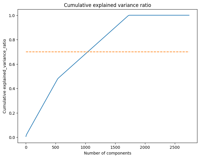
n_components_pca = np.argmax(cum_evr >= thresh) + 1
n_components_pca
## output: 1039
In this case, after plotting, it appears that 1039 components are required to explain 70% of the variance.
So, 1039 = the optimal number of principal components needed to capture the majority of variance in the data while reducing dimensionality.
Let’s reapply PCA with this specific number to transform both the training and testing datasets:
pca = PCA(n_components = n_components_pca)
X_train_pca = pca.fit_transform(X_train_scaled)
X_test_pca = pca.transform(X_test_scaled)
This transformation results in new training and testing sets that are now reduced in dimensionality but still capture the essence of the original datasets!
Decision tree
We start our exploration of decision tree classifiers by setting up a basic model using the default parameters.
clf = tree.DecisionTreeClassifier(random_state = 42)
clf.fit(X_train_pca, y_train)
Here we can print out the entire tree.
dot_data = tree.export_graphviz(clf, out_file = None)
graph = pydotplus.graph_from_dot_data(dot_data)
img = Image(graph.create_png())
img
It shows the decision paths from the root to the leaves:
Next, we evaluate the model on the test dataset to assess its accuracy. Using this tree to predict test data, we get the following:
y_pred = clf.predict(X_test_pca)

test_accuracy = accuracy_score(y_test, y_pred)
print(f"The test accuracy with basic decision tree is {test_accuracy}")
The test accuracy with basic decision tree is 0.9925464916558875
The reported accuracy from the basic decision tree is impressively high, at approximately 99.25%.
To further assess the model's performance, we analyze the confusion matrix:
cm = confusion_matrix(y_test, y_pred)

plt.figure(figsize=(8, 6))
p = sns.heatmap(pd.DataFrame(cm), annot=True, cmap="YlGnBu", fmt='g')
plt.title('Confusion Matrix', y=1.1)
plt.ylabel('Actual Label')
plt.xlabel('Predicted Label')
plt.show()
Optimizing Decision Tree Depth
To improve the decision tree model, we use cross-validation to determine the optimal tree depth.
parameters = {'max_depth': range(3, 15)}
clf = GridSearchCV(tree.DecisionTreeClassifier(), parameters, n_jobs = -1)
clf.fit(X = X_train_pca, y = y_train)

tree_model = clf.best_estimator_

print(f"The best parameter is {clf.best_params_} and the corresponding train score is {clf.best_score_}")
The best parameter is {'max_depth': 14} and the corresponding train score is 0.9943524447559969
We proceed to retrain our decision tree classifier using this optimized depth:
clf = tree.DecisionTreeClassifier(max_depth = 14)
clf.fit(X_train_pca, y_train)

y_pred = clf.predict(X_test_pca)

test_accuracy = accuracy_score(y_test, y_pred)
print(f"The test accuracy with best max depth decision tree is {test_accuracy}")
The test accuracy with best max depth decision tree is 0.9932992641913526
The corresponding decision tree is a more balanced tree and the testing accuracy is higher than the decision tree above.
dot_data = tree.export_graphviz(clf, out_file = None)
graph = pydotplus.graph_from_dot_data(dot_data)
img = Image(graph.create_png())
img
Updated confusion matrix:
cm = confusion_matrix(y_test, y_pred)
plt.figure(figsize=(8, 6))
p = sns.heatmap(pd.DataFrame(cm), annot=True, cmap="YlGnBu", fmt='g')
plt.title('Confusion Matrix', y=1.1)
plt.ylabel('Actual Label')
plt.xlabel('Predicted Label')
plt.show()
We can also plot the ROC curve:
fpr, tpr, thresholds = roc_curve(y_test, y_pred)

## plot the roc curve
plt.figure(figsize=(8, 6))
plt.plot([0,1], [0,1],'b--')
plt.plot(fpr, tpr, color = 'orange')
plt.xlabel('False Positive Rate')
plt.ylabel('True Positive Rate')
plt.title('Receiver Operating Characteristic Curve')
plt.show()
Observe that our decision tree analysis demonstrates the effectiveness of fine-tuning. Both the basic and optimized decision trees perform exceptionally well, which means there is great potential of using PCA-transformed features in classification tasks.
This analysis sets the stage for exploring more complex ensemble methods or different classifiers to see if performance can be enhanced further, following more steps below:
Bagging
Bagging is basically training multiple models on different subsets of the training dataset and then averaging their predictions to improve stability and accuracy.
Now we use bagging with decision tree classifier.
t = tree.DecisionTreeClassifier(random_state = 22)
bag = BaggingClassifier(estimator = t, n_jobs = -1)
bag = bag.fit(X_train_pca, y_train.values.ravel())

y_pred = bag.predict(X_test_pca)

test_accuracy = accuracy_score(y_test, y_pred)
print(f"The test accuracy with basic bagging (using decision tree) is {test_accuracy}")
The test accuracy with basic bagging (using decision tree) is 0.9952077016052079
99.52%. demonstrates the effectiveness of bagging in reducing variance and avoiding overfitting.
The confusion matrix and the ROC curve are as follows:

And ROC curve is

The confusion matrix and the ROC curve shows us the model's high performance.
K Nearest Neighbor (KNN)
Next, let’s explore the K Nearest Neighbor (KNN) classifier, a simple method that classifies new cases based on a similarity measure (aka distance functions).
We first start with the basic KNN:
clf = KNeighborsClassifier(n_neighbors = 3, n_jobs = -1)
clf.fit(X_train_pca, y_train.values.ravel())

y_pred = clf.predict(X_test_pca)

test_accuracy = accuracy_score(y_test, y_pred)
print(f"The test accuracy with basic bagging (using decision tree) is {test_accuracy}")
Optimizing KNN Parameters
To optimize the KNN classifier, we do a grid search to find the ideal number of neighbors.
Now we use cross validation to decide the best number of neighbors.
params = {'n_neighbors': np.arange(1, 10, 2)}

clf = GridSearchCV(KNeighborsClassifier(), params, cv = 5, n_jobs = -1)
clf.fit(X_train_pca, y_train.values.ravel())

print(f"The best parameter is {clf.best_params_} and the corresponding train score is {clf.best_score_}")
The best parameter is {'n_neighbors': 1} and the corresponding score is 0.9929105088693813
clf = KNeighborsClassifier(n_neighbors = 1, n_jobs = -1)
clf.fit(X_train_pca, y_train.values.ravel())

y_pred = clf.predict(X_test_pca)

test_accuracy = accuracy_score(y_test, y_pred)
print(f"The test accuracy for KNN with best number of neighbors is {test_accuracy}")
The test accuracy for KNN with best number of neighbors is 0.9939566148561251, demonstrating high true positive rates and low false positive rates.

ROC curve indicates an excellent performance:
fpr, tpr, thresholds = roc_curve(y_test, y_pred)

## plot the roc curve
plt.figure(figsize=(8, 6))
plt.plot([0,1], [0,1],'b--')
plt.plot(fpr, tpr, color = 'orange')
plt.xlabel('False Positive Rate')
plt.ylabel('True Positive Rate')
plt.title('Receiver Operating Characteristic Curve')
plt.show()
Discriminant Analysis
Linear Discriminant Analysis (LDA) is another technique we experimented.
LDA aims at finding a new axis that maximizes the separation between multiple classes.
LDA
from sklearn.discriminant_analysis import LinearDiscriminantAnalysis as LDA
from sklearn.discriminant_analysis import QuadraticDiscriminantAnalysis as QDA

clf = LDA(solver = 'lsqr')
clf.fit(X_train_pca, y_train.values.ravel())

y_pred = clf.predict(X_test_pca)

test_accuracy = accuracy_score(y_test, y_pred)
print(f"The test accuracy with LDA is {test_accuracy}")

## The test accuracy with LDA is 0.9929705888589665
Initially, LDA provides an accuracy of about 99.30%.
Optimizing LDA with Cross Validation
Now we use cross validation with LDA to find the optimal shrinkage parameter.
params = {'shrinkage': [0.1, 0.25, 0.5, 0.75, 1]}

clf = GridSearchCV(LDA(solver = 'lsqr'), params, cv = 5, n_jobs = -1)
clf.fit(X_train_pca, y_train.values.ravel())

print(f"The best parameter is {clf.best_params_} and the corresponding train score is {clf.best_score_}")
The best parameter is {'shrinkage': 0.25} and the corresponding train score is 0.992825693725328
Optimal results are achieved with a shrinkage of 0.25, slightly improving the accuracy to approximately 99.32%.
This parameter helps us regularize the LDA model, particularly handy when dealing with multicollinearity or multiple predictor variables.
clf = LDA(solver = 'lsqr', shrinkage = 0.25)
clf.fit(X_train_pca, y_train.values.ravel())

y_pred = clf.predict(X_test_pca)

test_accuracy = accuracy_score(y_test, y_pred)
print(f"The test accuracy with LDA is {test_accuracy}")

## The test accuracy with LDA is 0.9932462520409678

Both showcase effectiveness in classifying phishing URLs with high accuracy.
Quadratic Discriminant Analysis (QDA)
We also test Quadratic Discriminant Analysis (QDA), which allows for non-linear separation between classes.
clf = QDA()
clf.fit(X_train_pca, y_train.values.ravel())

y_pred = clf.predict(X_test_pca)

test_accuracy = accuracy_score(y_test, y_pred)
print(f"The test accuracy with LDA is {test_accuracy}")

## The test accuracy with LDA is 0.9796857439725185
However, QDA does not perform as well as LDA in this instance, with an accuracy around 97.97%. This suggests that the linear assumptions of LDA are sufficient for this dataset, and the more complex models might be overfitting or too sensitive to the specific data structure of our PCA-transformed features.
Hence, based on the test accuracy, LDA is more suitable than QDA in this case.
Support Vector Machine (SVM)
Support Vector Machines (SVMs) are renowned for their ability to handle high-dimensional data effectively.
from sklearn.svm import SVCFirst we fit a Support Vector Classifier to the data with regularization parameter C of 1.0 and a linear kernel.
svc = SVC(C = 1, kernel = 'linear')
svc = svc.fit(X_train_pca, y_train.values.ravel())

y_pred = svc.predict(X_test_pca)

test_accuracy = accuracy_score(y_test, y_pred)
print(f"The test accuracy with basic SVM is {test_accuracy}")
The test accuracy with basic SVM is 0.9967768612566 - an exceptionally high test accuracy.
To further analyze the performance, we visualize the confusion matrix and the Receiver Operating Characteristic (ROC) curve:
cm = confusion_matrix(y_test, y_pred)

plt.figure(figsize=(8, 6))
p = sns.heatmap(pd.DataFrame(cm), annot=True, cmap="YlGnBu", fmt='g')
plt.title('Confusion Matrix', y=1.1)
plt.ylabel('Actual Label')
plt.xlabel('Predicted Label')
plt.show()

fpr, tpr, thresholds = roc_curve(y_test, y_pred)

## plot the roc curve
plt.figure(figsize=(8, 6))
plt.plot([0,1], [0,1],'b--')
plt.plot(fpr, tpr, color = 'orange')
plt.xlabel('False Positive Rate')
plt.ylabel('True Positive Rate')
plt.title('Receiver Operating Characteristic Curve')
plt.show()
The confusion matrix reveals a high number of correct predictions with very few false positives and negatives. Good news.

ROC curve approaches the top left corner, meaning an excellent model performance!
Exploring SVM with RBF Kernel
Now we explore the SVM with a radial basis function (RBF) kernel, which can handle non-linear data distributions:
svc = SVC(C = 1, kernel = 'rbf')
svc = svc.fit(X_train_pca, y_train.values.ravel())

y_pred = svc.predict(X_test_pca)

test_accuracy = accuracy_score(y_test, y_pred)
print(f"The test accuracy with basic SVM is {test_accuracy}")
The test accuracy with basic SVM is 0.9910515490150342

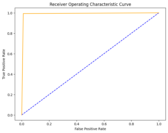
The confusion matrix for the RBF model shows slightly more misclassifications than the linear model, which is also reflected in the ROC curve.
Conclusion on SVM Performance
The comparative analysis between linear and RBF kernels in SVM shows the importance of choosing the right kernel based on the data's characteristics.
In our specific case, the simpler linear kernel proved more effective, which shows us an interesting observation that more complex models are not always superior!
Artificial Neural Networks Classification
Introduction to the ANN Architecture
The ANN has three types of layers: the input layer, the hidden layers, and the output layer. Initially, the network weights are assigned randomly. As input is fed into the input layer, it progresses forward, with each subsequent hidden layer receiving the input, modified by these weights. This process continues until it reaches the output layer, where a result is produced. This result is then compared to the actual value, triggering the backpropagation algorithm to adjust the network's weights and improve future results. The neurons in each layer facilitate this learning process. Each neuron contains an activation function that determines whether and how to transmit its received signal based on the input from the previous layer. We'll explore activation functions in greater detail shortly.
](https://raw.githubusercontent.com/jimyy23/pennfish-hugo/refs/heads/master/content/post/report/Untitled_45.png)
Source: https://www.sciencedirect.com/topics/earth-and-planetary-sciences/artificial-neural-network
Here’s a breakdown of the steps involved in this process:
- Assign random weights to all linkages to initiate the algorithm.
- Compute the activation rate of hidden nodes using the inputs and their linkages from the input layer.
- Determine the activation rate of output nodes, using the activation rates of hidden nodes and their linkages to the output.
- Calculate the error rate at the output node and adjust the linkages between hidden and output nodes to minimize this error.
- Propagate the error back from the output nodes to the hidden nodes, recalibrating the linkages between the input and hidden nodes.
- Repeat the process until the convergence criteria are met.
- Evaluate using the final linkage weights to determine the activation rate of the output nodes.
Split Data to Train, Validation, and Test
We will use the training set to fit the model, the validation set to tune the parameters (starting with the baseline model first) and the testing set for the final evaluation.
For the purpose of this project, we will use 70% for training, 15% for validation and 15% for testing.
## Set the ratios for train, validation and test
train_ratio = 0.7
validation_ratio = 0.15
test_ratio = 0.15

## we can set the seed 42 for reproducibility
random_state= 42

## Split the data into train, validation and test
X_train, X_test, y_train, y_test = train_test_split(df_features_encoded,
                                                    df_target,
                                                    test_size=1 - train_ratio,
                                                    random_state=random_state)

X_val, X_test, y_val, y_test = train_test_split(X_test,
                                                y_test,
                                                test_size=test_ratio/(test_ratio + validation_ratio),
                                                random_state=42)

## get shapes
print("Datasets after splitting:\n")
print(f"X_train: {X_train.shape}")
print(f"X_val: {X_val.shape}")
print(f"X_test: {X_test.shape}")
Datasets after splitting:
- X_train: (165056, 2740)
- X_val: (35369, 2740)
- X_test: (35370, 2740)
Feature Scaling
We don't want an independent variable to dominate the others in the model. So, we will scale the features to standardize the range of independent features of data. It also makes sure the gradient descent used in training converges more efficiently.
scaler = StandardScaler()
X_train = scaler.fit_transform(X_train)
X_val = scaler.transform(X_val)
X_test = scaler.transform(X_test)
Using ANN for Binary Classification: The Baseline Model
Let’s first set some parameters:
- input_shape: 2740 - number of input features each input example has.
- n_batch_size: 1650 - how many rows/instances of data the network processes at once (in training)
- n_steps_per_epoch: 100 - number of batches or steps the model trains on in each epoch (i.e., how many times the model will update its weights per epoch)
- n_validation_steps: 21 - and for the for the validation dataset
- n_epochs: 25 - umber of steps (batches) to evaluate the test set
input_shape = X_train.shape[1]

## num of samples per mini-batch of training data
## smaller batch size means noiser gradient, but can speed up training
n_batch_size = 100
n_steps_per_epoch = int(X_train.shape[0] / n_batch_size)
n_validation_steps = int(X_val.shape[0] / n_batch_size)
n_test_steps = int(X_test.shape[0] / n_batch_size)

## number of epochs is how often a complete
## run through the training data is performed
n_epochs = 25

print(f"input_shape: {input_shape}")
print(f"n_batch_size: {n_batch_size}")
print(f"n_steps_per_epoch: {n_steps_per_epoch}")
print(f"n_validation_steps: {n_validation_steps}")
print(f"n_test_steps: {n_test_steps}")
print(f"n_epochs: {n_epochs}")
Build the Baseline Model
Let’s initialize the layers, neurons, activation functions, and finally compile the model with a loss function and optimizer.
Here, we used 2 fully connected layers with 16 neurons each. Because this is a binary classification problem, the output layer has 1 neuron and uses a sigmoid activation function.
Hidden layers:
For the hidden layers, we use ReLU function. ReLU works in a way that its outputs the input directly if it is positive; otherwise, it outputs zero. It’s simple, so this makes ReLU very straightforward and efficient computationally. Specifically it prevents our activation levels from being too high or too low (which would be problematic with some other functions that squish values into a tiny range) so the data is generates is more useful for our purpose.
Output layer:
The sigmoid function squishes any real value into range between 0 and 1. Think of it a kind of translator that takes a wide range of input numbers and converts them into a language of probabilities. Handy when we need to predict probabilities for classification tasks like this one.
from keras import layers, models

model = models.Sequential([
    layers.Input(shape=(input_shape,)),

        # 2 fully connected layers with 16 neurons each
        model.add(layers.Dense(16, activation='relu'))
        model.add(layers.Dense(16, activation='relu'))

        # because this is a binary classification problem,
        # the output layer has 1 neuron and uses a sigmoid activation function
        model.add(layers.Dense(1, activation='sigmoid'))
])

model.summary()
Here is the layer structure:
Model: "sequential"
┏━━━━━━━━━━━━━━━━━━━━━━━━━━━━━━━━━┳━━━━━━━━━━━━━━━━━━━━━━━━┳━━━━━━━━━━━━━━━┓
┃ Layer (type)                    ┃ Output Shape           ┃       Param # ┃
┡━━━━━━━━━━━━━━━━━━━━━━━━━━━━━━━━━╇━━━━━━━━━━━━━━━━━━━━━━━━╇━━━━━━━━━━━━━━━┩
│ dense (Dense)                   │ (None, 16)             │        43,856 │
├─────────────────────────────────┼────────────────────────┼───────────────┤
│ dense_1 (Dense)                 │ (None, 16)             │           272 │
├─────────────────────────────────┼────────────────────────┼───────────────┤
│ dense_2 (Dense)                 │ (None, 1)              │            17 │
└─────────────────────────────────┴────────────────────────┴───────────────┘
 Total params: 44,145 (172.44 KB)
 Trainable params: 44,145 (172.44 KB)
 Non-trainable params: 0 (0.00 B)
Compile the model:
## Configure the model for training
model.compile(loss='binary_crossentropy',
                optimizer='adam',
                metrics=['accuracy'])
Let’s also store the callbacks, so we may use the model later again.
## store checkpoints
checkpoint_dir = f'./{checkpoint_no}'
if not os.path.exists(checkpoint_dir):
    os.makedirs(checkpoint_dir)

keras_callbacks = [
    ModelCheckpoint(
        filepath=os.path.join(checkpoint_dir, model_name),
        monitor='val_loss',
        save_best_only=True,
        mode='auto'
    )
]
Fit the Baseline Model
history = model.fit(
    X_train,
    y_train,
    epochs=n_epochs,
    batch_size=n_batch_size,
    validation_data=(X_val, y_val),
    steps_per_epoch=n_steps_per_epoch,
    validation_steps=n_validation_steps,
    callbacks=keras_callbacks
)
Wait until all the epochs have been finished:
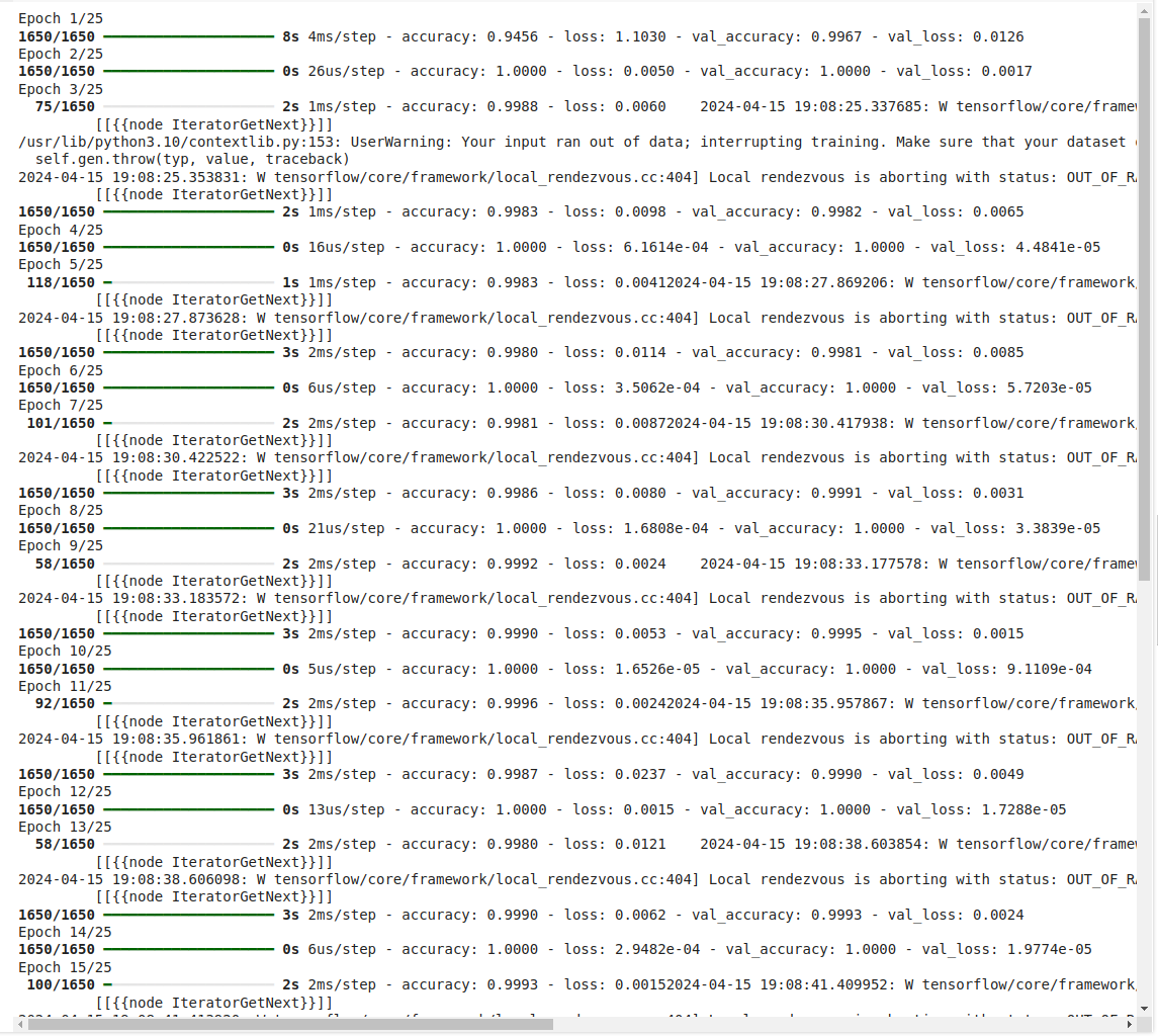
Get the best model values
## Get the best model values
df_history = pd.DataFrame(history.history)
df_history['epoch'] = df_history.index + 1
df_history = df_history[['epoch'] + [col for col in df_history.columns if col != 'epoch']]
df_history.to_csv(f"{checkpoint_no}/history_df_{model_name}.csv")
df_history.head()

values_of_best_model = df_history.loc[df_history.val_loss.idxmin()]
values_of_best_model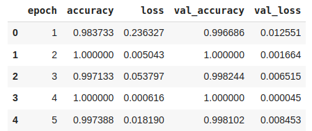
values_of_best_model:
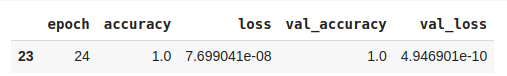
Also save the class assignments, so we can use them later.
class_assignment = {'phishing': 0, 'legitimate': 1}

df_class_assignment = pd.DataFrame(list(class_assignment.items()), columns=['Category', 'Class'])
df_class_assignment.to_csv(f"{checkpoint_no}/class_assignment_df_{model_name}.csv")

## save the scaler
with open(f'{checkpoint_no}/scaler.pkl', 'wb') as f:
    pk.dump(scaler, f)
Validation
Going ahead to validation, where we will compare the models predictions on the validation set. We are going to get both the accuracy (how often the model's predictions match the true labels) and loss (how far off the predictions are from the actual results).
accuracy = history.history['accuracy']
validation_accuracy = history.history['val_accuracy']
loss = history.history['loss']
val_loss = history.history['val_loss']
epochs = range(1, len(accuracy) + 1)

plt.figure(figsize=(12, 6))
plt.plot(epochs, accuracy, 'bo', label='Training acc')
plt.plot(epochs, validation_accuracy, 'b', label='Validation acc')
plt.title('Training and validation accuracy')
plt.legend()

plt.figure(figsize=(12, 6))
plt.plot(epochs, loss, 'bo', label='Training loss')
plt.plot(epochs, val_loss, 'b', label='Validation loss')
plt.title('Training and validation loss')
plt.legend()

plt.show()
Plot the training accuracy (accuracy) and validation accuracy (validation_accuracy) are plotted against the number of epochs:
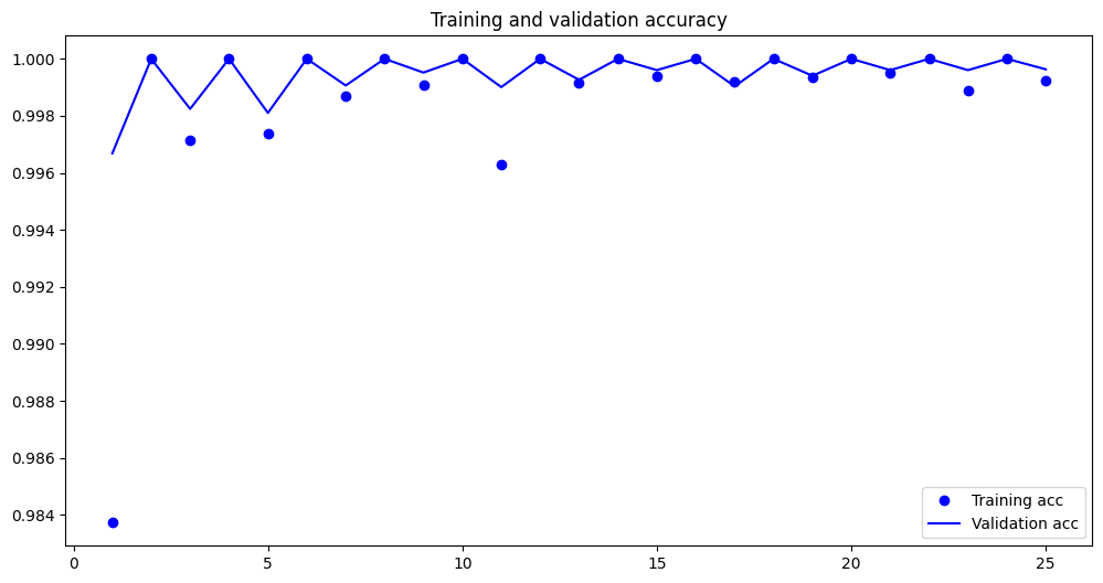
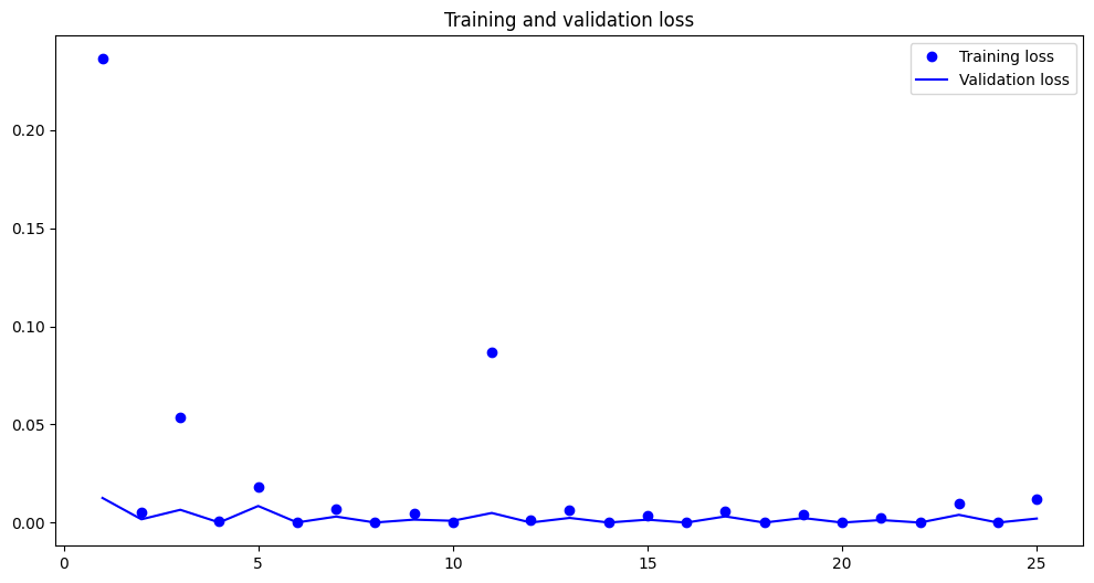
Not much overfitting observed.
Test the Baseline Model
## Loading the saved model
model_reloaded = load_model(f"{checkpoint_no}/{model_name}")
root_directory = os.getcwd()
checkpoint_dir = os.path.join(root_directory, checkpoint_no)
saved_model_name = os.path.join(checkpoint_dir, f"{model_name}.keras")
model_reloaded.save(saved_model_name)

## Delete the saved model
saved_model_path = os.path.join(checkpoint_dir, model_name)
shutil.rmtree(saved_model_path, ignore_errors=True)

## load the best model
best_model = load_model(saved_model_name)
test_score, test_accuracy = best_model.evaluate(X_test, y_test, n_test_steps)
print('Test Accuracy:', test_accuracy)101/101 ━━━━━━━━━━━━━━━━━━━━ 0s 2ms/step - accuracy: 0.9997 - loss: 0.0022
Test Accuracy: 0.9996324777603149The test accuracy is pretty high with a very low loss value. Let’s proceed with the following steps to further improve the model.
Improve the ANN Model by Tuning the ANN and Avoiding Overfitting
Set Parameters
Instead of an arbitrary n_batch_size, here we use 1% of the training data. Smaller batch sizes can introduce more noise into the gradient descent process.
input_shape = X_train.shape[1]
sample_size = X_train.shape[0]

## num of samples per mini-batch of training data
## smaller batch size means noiser gradient, but can speed up training
n_batch_size = int(0.01 * sample_size) # here we use 1% of the training data

n_steps_per_epoch = int(X_train.shape[0] / n_batch_size)
n_validation_steps = int(X_val.shape[0] / n_batch_size)
n_test_steps = int(X_test.shape[0] / n_batch_size)

## number of epochs is how often a complete
## run through the training data is performed
n_epochs = 25

print(f"input_shape: {input_shape}")
print(f"sample_size: {sample_size}")
print(f"n_batch_size: {n_batch_size}")
print(f"n_steps_per_epoch: {n_steps_per_epoch}")
print(f"n_validation_steps: {n_validation_steps}")
print(f"n_test_steps: {n_test_steps}")
print(f"n_epochs: {n_epochs}")
Implementing Early Stoping
We implement early stopping to prevent overfitting. What is does is automatically stopping the training process when the validation score stops improving.
early_stopping = EarlyStopping(monitor='val_loss', patience=10)Implementing a Learning Rate Schedule
Instead of a fixed lr let's use a learning rate schedule. This will reduce the learning rate when as training goes on.
reduce_lr = ReduceLROnPlateau(monitor='val_loss', factor=0.2, patience=5, min_lr=0.001)Implementing the Weight Regularization
A learning rate schedule adjusts the learning rate over time. It reduces the learning rate if the validation loss stops improving.
regularizer=regularizers.l2(0.001)Build the Model
Here is where we can rename our model.
For this project, let's name our model URL_ANN_2FC_F16_16_epoch_25 because of the parameters we set above.
checkpoint_no = 'checkpoint_1_ANN'
model_name = 'URL_ANN_2FC_F16_16_epoch_25.keras'
Note that Kera requires models to have a filename ending in .keras.
Implementing Dropout Layers
Incorporate the changes we have made, and also implement some dropout layers.
Dropout is a regularization technique used to prevent overfitting. The dropout layer randomly sets a fraction p of the input units to 0 at each update during training time, which helps us to make the activation of the neurons sparse, thus reducing overfitting.
We have tried setting them at different levels from 0.1 to 0.5. Here in the example below, we set p to 0.5, which means we randomly exclude half of the neuron outputs from each update cycle.
Note that in some cases setting it as high as 0.5 or above might lead to underfitting.
def create_model():
    model = models.Sequential()
    model.add(layers.Input(shape=(input_shape,)))

    # 2 fully connected layers with 16 neurons each:
    model.add(layers.Dense(16,
                        kernel_regularizer=regularizer,
                        activation='relu'))

    # add some dropouts to prevent overfitting
    model.add(layers.Dropout(0.5))

    model.add(layers.Dense(16,
                        kernel_regularizer=regularizer,
                        activation='relu'))

    # add some dropouts to prevent overfitting
    model.add(layers.Dropout(0.5))

    # because this is a binary classification problem,
    # the output layer has 1 neuron and uses a sigmoid activation function
    model.add(layers.Dense(1, activation='sigmoid'))

    # Configure the model for training
    model.compile(loss='binary_crossentropy',
                optimizer='adam',
                metrics=['accuracy'])

    return model
Same as before:
model = create_model()
model.summary()
Model: "sequential"
┏━━━━━━━━━━━━━━━━━━━━━━━━━━━━━━━━━━━━━━┳━━━━━━━━━━━━━━━━━━━━━━━━━━━━━┳━━━━━━━━━━━━━━━━━┓
┃ Layer (type) ┃ Output Shape ┃ Param # ┃
┡━━━━━━━━━━━━━━━━━━━━━━━━━━━━━━━━━━━━━━╇━━━━━━━━━━━━━━━━━━━━━━━━━━━━━╇━━━━━━━━━━━━━━━━━┩
│ dense (Dense) │ (None, 16) │ 43,856 │
├──────────────────────────────────────┼─────────────────────────────┼─────────────────┤
│ dropout (Dropout) │ (None, 16) │ 0 │
├──────────────────────────────────────┼─────────────────────────────┼─────────────────┤
│ dense_1 (Dense) │ (None, 16) │ 272 │
├──────────────────────────────────────┼─────────────────────────────┼─────────────────┤
│ dropout_1 (Dropout) │ (None, 16) │ 0 │
├──────────────────────────────────────┼─────────────────────────────┼─────────────────┤
│ dense_2 (Dense) │ (None, 1) │ 17 │
└──────────────────────────────────────┴─────────────────────────────┴─────────────────┘
Total params: 44,145 (172.44 KB)
Trainable params: 44,145 (172.44 KB)
Non-trainable params: 0 (0.00 B)Then, we set up the callbacks following the same steps. Codes are omitted here.
Fit the Model
history = model.fit(X_train, y_train,
                    epochs=n_epochs,
                    batch_size=n_batch_size,
                    validation_data=(X_val, y_val),
                    steps_per_epoch=n_steps_per_epoch,
                    validation_steps=n_validation_steps,
                    callbacks=[keras_callbacks, early_stopping, reduce_lr])
## Get the best model values
df_history = pd.DataFrame(history.history)
df_history['epoch'] = df_history.index + 1
df_history = df_history[['epoch'] + [col for col in df_history.columns if col != 'epoch']]
df_history.to_csv(f"{checkpoint_no}/history_df_{model_name}.csv")
df_history.head()
values_of_best_model = df_history.loc[df_history.val_loss.idxmin()]
values_of_best_modelepoch 12.000000
accuracy 1.000000
loss 0.048962
val_accuracy 1.000000
val_loss 0.022055
learning_rate 0.001000
Name: 11, dtype: float64Validation
accuracy = history.history['accuracy']
validation_accuracy = history.history['val_accuracy']
loss = history.history['loss']
val_loss = history.history['val_loss']
epochs = range(1, len(accuracy) + 1)

plt.figure(figsize=(12, 6))
plt.plot(epochs, accuracy, 'bo', label='Training acc')
plt.plot(epochs, validation_accuracy, 'b', label='Validation acc')
plt.title('Training and validation accuracy')
plt.legend()

plt.figure(figsize=(12, 6))
plt.plot(epochs, loss, 'bo', label='Training loss')
plt.plot(epochs, val_loss, 'b', label='Validation loss')
plt.title('Training and validation loss')
plt.legend()

plt.show()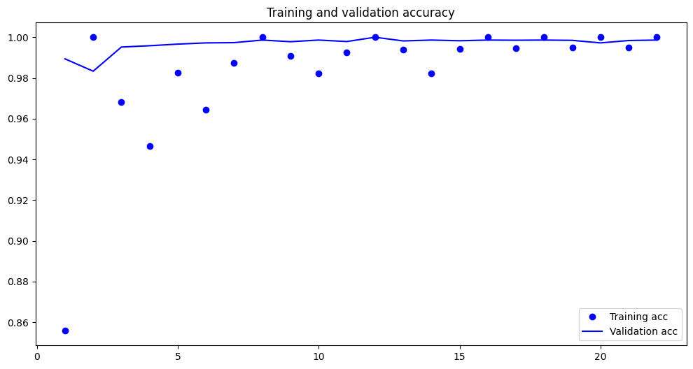
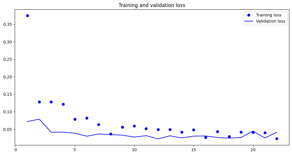
The validation loss generally remains low and close to the training loss, which suggests that the model is not overfitting and has learned the underlying patterns in the data well.
Testing the Model
test_score, test_accuracy = best_model.evaluate(X_test, y_test, n_test_steps)
print(f"Test Score: {test_score}")
print(f"Test Accuracy: {test_accuracy}")
1685/1685 ━━━━━━━━━━━━━━━━━━━━ 3s 2ms/step - accuracy: 0.9988 - loss: 0.0276
Test Score: 0.02890169993042946
Test Accuracy: 0.9984450340270996The model is performing very well with high accuracy and low loss on both the training and validation datasets.
Make Predictions
## Make predictions
y_pred_prob = best_model.predict(X_test)

y_pred_prob
array([[1.2841106e-06],
[9.9997938e-01],
[1.0000000e+00],
...,
[6.7629302e-09],
[1.5825824e-06],
[9.9999905e-01]], dtype=float32)We need to convert the predictions to binary values.
Let's use a threshold of 0.5. If the prediction is greater than 0.5, we will consider it as 1, otherwise 0.
y_pred = (y_pred_prob > 0.5).astype(int)Evaluation
Confusion Matrix
cm = confusion_matrix(y_test, y_pred)
plt.figure(figsize=(8, 6))
p = sns.heatmap(pd.DataFrame(cm), annot=True, cmap="YlGnBu", fmt='g')
plt.title('Confusion Matrix', y=1.1)
plt.ylabel('Actual Label')
plt.xlabel('Predicted Label')
plt.show()
Classification Report
print(classification_report(y_test, y_pred)) precision recall f1-score support
0 1.00 1.00 1.00 15090
1 1.00 1.00 1.00 20280
accuracy 1.00 35370
macro avg 1.00 1.00 1.00 35370
weighted avg 1.00 1.00 1.00 35370ROC Curve
Let's plot the ROC curve to see how well the model performs. The ROC curve plots the true positive rate (TPR) against the false positive rate (FPR) at diffrent values of threshold. The closer the curve follows the left-hand border and then the top border of the ROC space, the more accurate the test.
## calculate the probabilities using the classifier
y_pred_proba = best_model.predict(X_test)[:,0]

## calculate the roc curve
fpr, tpr, thresholds = roc_curve(y_test, y_pred_proba)

## plot the roc curve
plt.figure(figsize=(8, 6))
plt.plot([0,1],[0,1],'k--')
plt.plot(fpr,tpr, label='ANN')
plt.xlabel('False Positive Rate')
plt.ylabel('True Positive Rate')
plt.title('Receiver Operating Characteristic (ROC) Curve')
plt.legend(loc='lower right')
plt.show()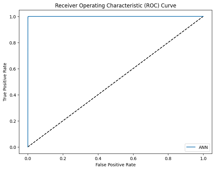
## area under the curve
print(f"ROC AUC Score: {roc_auc_score(y_test, y_pred_proba)}")
ROC AUC Score: 0.9998084438797851We observed that the AUC score is very close to 1, which is a good sign that the model is doing a good job to classify the URLs to be phishing or not.
Conclusion of ANN
Overall, the model is performing very well with high accuracy and low loss on both the training and validation datasets. The consistent high accuracy and low loss over epochs without a widening gap between training and validation metrics indicate that the model is stable and generalizes well.
Challenges
Our project applied the application of an artificial neural network (ANN) for the binary classification, which included developing a baseline model, tuning the ANN, preventing overfitting, building the model, and evaluating it. We modified the ANN model to achieve more accurate predictions of phishing websites.
We also applied Principal Component Analysis (PCA) to reduce the dimensionality of the data before applying it to a Support Vector Machine (SVM). Despite this, it still took a considerable amount of time to run (over an hour for a simple linear kernel SVM).
The large size of the data made cross-validation challenging; a simple 5-fold cross-validation with a few tuning parameters could take more than an hour.
To avoid system crashes, we used high-RAM machines to reduce boot-up and shutdown times, and to ensure smooth program launches and task executions.
We also used a T4 GPU as a hardware accelerator, which provides strong performance for mid-range machine learning tasks.
On average, each team member dedicated 20 hours to the project.
Conclusion
Our project started from the acquisition of data, preprocessing, exploratory analysis, and moving through to the model training phase.
The project applied logistic regression, PCA to reduce dimensionality, logistic regression with PCA, ridge regression, linear regression (unregularized), linear regression (unregularized) with PCA, random forest classifier, random forest regression, and decision tree classifier.
We also extend the scope to k-nearest neighbor, discriminant analysis, support vector machine (SVM), and artificial neural networks classification (ANN).
A significant emphasis was placed on evaluating different models to establish their efficacy in distinguishing between legitimate and phishing websites.
From our results, the machine learning models achieved very high accuracy, demonstrating their capability to generalize well on unseen data — particularly highlighted by the performance of the artificial neural networks and support vector machines, which not only provided robust classification metrics but also indicated low overfitting as evidenced by the minimal gap between training and validation losses.
Closing Notes
Overall, the project not only advances academic and practical understandings of phishing detection, but it also shows a potential approach for future research that could include more sophisticated algorithms and integration with real-time data systems. 🐟
Authors: Jim, Lucy, Qimeng, KK
References
- Dutta, A. (2021). Detecting phishing websites using machine learning technique. PLoS ONE, 16. https://doi.org/10.1371/journal.pone.0258361.
- Gastellier-Prevost, S., Granadillo, G., & Laurent, M. (2011). Decisive Heuristics to Differentiate Legitimate from Phishing Sites. 2011 Conference on Network and Information Systems Security, 1-9. https://doi.org/10.1109/SAR-SSI.2011.5931389.
- Levy, E. (2004). Interface Illusions. IEEE Secur. Priv., 2, 66-69. https://doi.org/10.1109/MSP.2004.104.
- Michael Fuchs Python. (2021, February 16). NN – Artificial neural network for binary classification. https://michael-fuchs-python.netlify.app/2021/02/16/nn-artificial-neural-network-for-binary-classification/#encoding